1. Lorentzian Harmonic Flow (⚡LHF) Indicator Description
A market analysis tool based on curved-time theory and historical memory
1.1 Indicator Concept
LHF (Lorentzian Harmonic Flow) posits that market time doesn’t tick evenly like a clock. When volatility spikes, time is “compressed” — a week’s worth of action can unfold in minutes. When the market ranges, time “expands” — price oscillates with no clear trend.
LHF applies the Lorentz formula from Einstein’s relativity to compute the gamma (γ) factor — representing the degree of time compression/expansion:
• v (velocity): Trend speed — measured by distance price travels over N bars, normalized by ATR
• c (speed of market): The market’s “speed limit” — derived from realized volatility + sudden bursts
• γ: When γ ≈ 1 → normal time; γ > 2 → time compression, use shorter lenses to capture information
Core principle: The market has its own “harmonic structure” (rhythm) and “memory.” When the present resembles the past (similar flow, gamma, entropy, etc.), future outcomes tend to echo prior scenarios.
1.2 Indicator Features
On-chart visuals:
- Flow River Bands (Flow Upper/Lower): Two faint green/red bands around price reflecting current “Harmonic Flow” (HFL). Bands widening → stronger flow; narrowing → weaker flow.
- Compression Cloud: A faint orange area around price that widens when TCI is high (time compression) — signaling energy “stored” like a compressed spring.
- Prediction Arc: A curve projecting forward from current price, blending flow velocity (HFL_vel), acceleration (HFL_acc), and memory bias (mem_bias). Green → bullish drift; red → bearish drift.
- LONG/SHORT Signal Markers: Small ▲ (LONG) or ▼ (SHORT) triangles plot when conditions align: squeeze release, strong flow, correct acceleration, and supportive memory.
- Background Aura: Light green/red backdrop showing overall bias from the final_score — context only, not an entry signal.
Dashboard:
- Gamma (γ): Time-compression factor. Yellow when high → market accelerating.
- TCI (Temporal Compression Index): Compression index = base_length / adaptive_length. TCI > 1 → time is compressed.
- v/c: Velocity to speed-limit ratio. Red when v/c > 0.7 → nearing the market’s “speed of light.”
- Entropy: Market disorder. High → harder to forecast; be cautious.
- HFL (Harmonic Flow): Positive → bullish bias; negative → bearish bias.
- HFL_acc: Flow acceleration. Yellow when elevated → flow strengthening in its direction.
- Mem Bias: Historical memory tilt. Green/red depending on past outcomes.
- Assurance: Memory confidence. Yellow when > 1 → many similar historical scenarios.
- Squeeze: Volatility compression state (BB < KC). 🔴 ON → compressing; 🟢 RELEASE → just released.
- Breakout P: Breakout probability (0–100%). Green when > 70%.
- Score: Composite of flow and memory. Green → bullish; red → bearish.
- Signal: 🚀 LONG / 🔻 SHORT / ⚪ NEUTRAL — final verdict.
Heat Map (memory map):
- 2D table showing “resonance” between present and past.
- X-axis: Memory age (left = recent, right = distant).
- Y-axis: Flow regime (top = strong bearish, middle = neutral, bottom = strong bullish).
- Color: Green = bullish past outcome; Red = bearish. Intensity = similarity.
- How to read: A dark green column in bullish flow (bottom) and recent age → memory suggests strong upside.
Alerts:
- Alerts on LONG signal, SHORT signal, or Squeeze Release.
- Configure TradingView notifications so you don’t miss signals.
1.3 How to Use the Indicator
Five-step analysis workflow:
- Step 1 — Set context: Check Gamma and TCI on the dashboard. If both are high → time is compressed, information arrives fast → prioritize short-term setups and use adaptive logic.
- Step 2 — Assess current state: Inspect HFL and HFL_acc. If HFL > 0 and HFL_acc > 0 → bullish pressure accelerating. If HFL < 0 and HFL_acc < 0 → bearish pressure accelerating.
- Step 3 — Consult memory: Read Mem Bias and Assurance. If Mem Bias aligns with HFL and Assurance is high → strong signal due to historical support.
- Step 4 — Check compression mechanics: Look at Squeeze and Breakout P. If Squeeze just RELEASED, Breakout P > 70%, and HFL/Mem Bias agree → high-quality setup.
- Step 5 — Make the trade decision: Use final_score as the “gate.” If score > 0.3 → strong long bias; < -0.3 → strong short bias. Place stops beyond the nearest pivot; target via Prediction Arc or Fibonacci.
Multi-timeframe usage:
- Higher TF (4H, Daily): Use Gamma, TCI, HFL slope to determine overall trend and regime (trending vs ranging).
- Lower TF (15M, 1H): Execute entries on HFL_acc spikes, squeeze releases, or when final_score crosses thresholds.
- Memory automatically captures cross-timeframe patterns — no special setup needed.
Sample trading strategies:
- LONG setup: Squeeze RELEASE + HFL > flow_threshold + HFL_acc > 0 + Mem Bias > 0 + Assurance > 1 + final_score > 0.3 → Enter long, stop below the nearest low.
- SHORT setup: Squeeze RELEASE + HFL < -flow_threshold + HFL_acc < 0 + Mem Bias < 0 + Assurance > 1 + final_score < -0.3 → Enter short, stop above the nearest high.
- Avoid trades when: Entropy high + Assurance low + Gamma near 1 (normal but chaotic market) → wait for clarity.
1.4 How the Indicator Works
A. Inputs and roles:
- base_len (Base Length, default 55): Baseline length under normal market conditions (γ ≈ 1). Serves as the “anchor” for adaptive_length = base_len / γ^power. Lower (21–34) → faster for volatile assets; higher (89–144) → stabler for slower assets.
- vel_len (Velocity Window, default 21): Bars used to compute trend speed (v). v = |close - close[vel_len]| / (vel_len × ATR). Shorter → more sensitive gamma; longer → steadier gamma.
- vol_len (Volatility Window, default 21): Bars to compute realized volatility (stdev of log returns) and burst (sudden changes in volatility). Used to compute c (speed of market).
- c_multiplier (Speed Multiplier, default 1.0): Multiplier for c. Lower → smaller c → v/c rises easily → gamma increases faster. Higher → larger c → harder to reach high gamma.
- short_ratio, mid_ratio, long_ratio (defaults 0.5, 1.0, 2.0): Split adapt_len into three horizons. Len_short = adapt_len × 0.5; Len_mid = adapt_len × 1.0; Len_long = adapt_len × 2.0.
- w_short, w_mid, w_long (defaults 0.4, 0.35, 0.25): Weights to blend three z-scores into HFL. Increase w_short → snappier HFL; increase w_long → smoother HFL.
- mem_size (Memory Size, default 256): Ring-buffer size for feature vectors and outcomes. Larger → remembers more past patterns → heavier CPU.
- k_neighbors (default 16): Number of nearest neighbors (k-NN) when fetching similar memories. Smaller → more reactive; larger → smoother.
- mem_fade (Memory Fade, default 0.95): Age decay factor. weight_age = mem_fade^age_bars. Lower (0.8–0.9) → prioritize recent; higher (0.95–0.99) → retain memory longer.
- squeeze_mult, flow_thr, accel_thr: Thresholds for squeeze (BB < KC × squeeze_mult), minimum flow, and minimum acceleration for signaling.
B. Main logic blocks and roles:
B1. Compute Gamma (γ) — Time compression factor:
- Log return: r = log(close / close[1])
- Realized volatility: rv = stdev(r, vol_len)
- Burst: burst = |rv - rv[1]|
- Speed of market: c = c_multiplier × (ema(rv) + 0.5 × ema(burst) + epsilon)
- Trend velocity: v = |close - close[vel_len]| / (vel_len × ATR)
- Relative velocity: v_rel = v / c
- Gamma: gamma = 1 / sqrt(1 - v_rel²), capped to [1, 10]
- Role: Gamma represents the market’s “time speed.” Rising gamma → time compresses → analysis must speed up.
B2. Adaptive Length (L) — Adjust the lens:
- adapt_len = base_len / gamma^power
- If auto_adapt = true, also adjust by entropy.
- Role: High gamma → smaller adapt_len → “shorter view” to keep up with an accelerating market.
B3. Lorentzian Smoothing — Build harmonic baselines:
- For each horizon (short, mid, long), scan up to max_kernel_len bars.
- Each bar i has weight: w_i = 1 / (1 + (d/gamma)²), with d = i / adapt_len
- Baseline: lw_h = Σ(w_i × price[i]) / Σ(w_i)
- Z-score: z_h = (close - lw_h) / ATR
- Role: Produce three z-scores (short, mid, long) representing price deviation from baseline across three lenses.
B4. HFL (Harmonic Flow) — Market flow:
- HFL = (w_short × z_short + w_mid × z_mid + w_long × z_long) / (w_short + w_mid + w_long)
- Role: HFL is the market “temperature” under curved time. Positive → bullish bias; negative → bearish bias.
B5. HFL_vel and HFL_acc — Flow dynamics:
- Velocity: HFL_vel = HFL - HFL[1]
- Acceleration: HFL_acc = HFL - 2×HFL[1] + HFL[2]
- Role: HFL_vel shows direction of change; HFL_acc captures curvature/turning — spikes often precede strong shifts.
B6. Entropy — Market disorder:
- Based on Shannon entropy of |log returns| distribution.
- entropy = -Σ(p_i × log(p_i)), where p_i is each bin’s share.
- Role: High → chaotic, low predictability. Low → more ordered, easier to analyze.
B7. Squeeze and TCI — Volatility compression:
- BB width = 2 × stdev(close, adapt_len)
- KC width = 2 × ATR(adapt_len)
- squeeze_on = (BB_width < KC_width × squeeze_mult)
- squeeze_rel = squeeze_on[1] and not squeeze_on (just exited squeeze)
- TCI: TCI = base_len / adapt_len
- Role: Squeeze = compressed spring → energy stored. TCI > 1 → time compressing. Together → anticipate bursts.
B8. K-NN Memory — Retrieve similar past scenarios:
-
Store: On each confirmed bar, push into ring buffer:
- Feature: [HFL, gamma, entropy, ema(rv), HFL_vel]
- Outcome: Forward returns at H5, H13, H34 (e.g., return after 5, 13, 34 bars)
-
Search: For current features, compute similarity to each neighbor:
- Per-dimension kernel: k(Δ) = 1 / (1 + Δ²)
- Similarity = product of kernels across 5 dims, with user-defined weights (feat_w_flow, feat_w_gamma, ...)
- Age fade: weight = mem_fade^age_bars
- Neighbor score: s_i = similarity_i × weight_age_i
-
Vote: Take k neighbors with highest scores.
- Mem Bias: Σ(s_i × outcome_i) / Σ(s_i) → weighted mean of forward returns
- Assurance: Σ(s_i) → total confidence mass
- Normalize: mem_bias_norm = tanh(mem_bias / (ATR × scale)) → map to [-1, 1]
- Role: Memory tells “what the past suggests now.” High assurance + mem_bias aligned with HFL → stronger conviction.
B9. Breakout Probability — Likelihood of burst:
- Energy = cap(TCI - 1, max=2) + |HFL_acc| × k + cap(gamma - 1, max=3) × k + cap(mem_assurance, max=2) × k
- Breakout_prob = sigmoid(energy) = 1 / (1 + exp(-energy))
- Role: Aggregates compression + acceleration + gamma + memory into 0–1. > 0.7 → high breakout odds.
B10. Final Score — Composite signal:
- Blend ratio: alpha_mem = 0.45 + 0.15 × (gamma - 1) → higher gamma increases memory weighting
- Final_score = (1 - alpha_mem) × tanh(HFL / (flow_thr × 1.5)) + alpha_mem × tanh(mem_bias_norm)
- Role: Combines present flow with memory bias. Higher gamma → trust memory more (as the market accelerates, past patterns matter more).
B11. Generate LONG/SHORT signals:
- Long: squeeze_rel + HFL > flow_thr + HFL_acc > accel_thr + mem_bias_norm > 0 + final_score > score_thr + distance from last signal > min_gap
- Short: squeeze_rel + HFL < -flow_thr + HFL_acc < -accel_thr + mem_bias_norm < 0 + final_score < -score_thr + gap > min_gap
- Role: Plot markers only with sufficient confluence and avoid signal spam.
C. Outputs mapped to visuals:
- HFL → Flow River: flow_up/flow_dn = close ± HFL × flow_scale. Plotted as green/red bands.
- TCI → Compression Cloud: comp_up/comp_dn = close × (1 ± (TCI-1) × 0.02). Plotted as orange region.
- HFL_vel, HFL_acc, mem_bias → Prediction Arc: pred_arc = close + v_price × dt + 0.5 × a_price × dt². Plots the forward curve.
- long_fire/short_fire → Markers: ▲/▼ above/below bars.
- final_score → Background Aura: Light green/red backdrop.
- Dashboard: Displays key variables (gamma, TCI, HFL, mem_bias, ...).
- Heat Map: 2D table from heat_w and heat_val arrays, split into age bins (X) and flow bins (Y).
Assume current bar: close=50000, ATR=500, base_len=55.
- Log return: r = log(50000/49800) ≈ 0.004
- rv = stdev(r, 21) ≈ 0.02; burst ≈ 0.001
- c = 1.0 × (ema(0.02) + 0.5 × ema(0.001)) ≈ 0.021
- v = |50000 - 48000| / (21 × 500) ≈ 0.19
- v_rel = 0.19 / 0.021 ≈ 9.05 (over limit, cap v_rel < 1 to avoid NaN)
- After capping: v_rel = 0.85 → gamma = 1 / sqrt(1 - 0.85²) ≈ 1.90
- adapt_len = 55 / 1.90^1.0 ≈ 29 bars → TCI = 55/29 ≈ 1.90 (time compression)
- Three horizons: Len_short ≈ 14, Len_mid ≈ 29, Len_long ≈ 58
- Lorentz kernel scan → z_short ≈ 1.2, z_mid ≈ 0.8, z_long ≈ 0.5
- HFL = (0.4×1.2 + 0.35×0.8 + 0.25×0.5) / 1.0 ≈ 0.885 (strong bullish bias)
- HFL_vel = 0.885 − 0.7 = 0.185; HFL_acc = 0.885 − 2×0.7 + 0.6 = 0.085 (positive → accelerating)
- Entropy ≈ 2.5 (moderate); squeeze_on = false, squeeze_rel = true (just released)
- K-NN finds 16 neighbors, mem_bias_norm ≈ 0.4 (bullish past), assurance ≈ 1.5 (high confidence)
- Breakout_prob = sigmoid(1.9 + 0.085×k + 0.9×k + 1.5×k) ≈ 0.75 (75% breakout odds)
- alpha_mem = 0.45 + 0.15×(1.9−1) = 0.585
- final_score = (1−0.585)×tanh(0.885/0.3) + 0.585×tanh(0.4) ≈ 0.65 (strong bullish bias)
- Long signal = true (conditions met) → Plot LONG marker ▲
- Prediction Arc = 50000 + (0.185×flow_scale)×10 + 0.5×(0.085×flow_scale)×100 ≈ 50500 (projects ~10 bars ahead)
Conclusion: With strong flow (HFL=0.885), positive acceleration, supportive memory, recent squeeze release, and high TCI → the indicator issues a high-confidence LONG. Dashboard shows Score=0.65 (green), Breakout P=75%, Signal=🚀 LONG ▲.


Use the analysis above + the code below to instruct AI to modify the indicator and turn it into a trading bot—no coding required!
How to do it here -> 👉ZERO2HERO👈
					//@version=5
indicator("Lorentzian Harmonic Flow - Temporal Market Dynamic ", shorttitle="⚡ LHF", overlay=true, max_labels_count=500, max_lines_count=500, max_bars_back=5000)

//==============================================================================
// ⚡ LORENTZIAN HARMONIC FLOW - TEMPORAL MARKET DYNAMICS
//==============================================================================
//
// 🌌 THEORETICAL FOUNDATION: MARKET TIME AS CURVED SPACETIME
//
// Traditional indicators treat time as linear and uniform—each bar weighted
// equally, each moment progressing at constant velocity. But markets don't
// behave this way. During explosive volatility, price action "compresses"
// weeks of movement into minutes. During consolidation, time "dilates" as
// price meanders without conviction.
//
// The Lorentzian Harmonic Flow (LHF Pro) treats this phenomenon literally,
// borrowing from Einstein's special relativity to model market time dilation.
//
// 🔬 THE LORENTZ TRANSFORMATION: FROM PHYSICS TO FINANCE
//
// In special relativity, the Lorentz gamma factor governs time dilation:
//
// γ = 1 / √(1 - v²/c²)
//
// Where:
// • v = velocity of an object (here: trend velocity, normalized by ATR)
// • c = speed of light (here: "speed of market" ~ realized volatility + bursts)
// • γ = time dilation factor (γ > 1 means time compresses)
//
// When trend velocity approaches market's "speed limit" (high vol), gamma
// spikes → time compresses → we use shorter lookback windows to capture
// the accelerated information flow. Conversely, in sleepy markets (v ≈ 0),
// gamma ≈ 1 and time flows normally.
//
// This isn't a metaphor—it's a quantitative framework that adapts every
// parameter to the market's intrinsic clock.
//
// 🎼 HARMONIC FLOW: MULTI-HORIZON RESONANCE IN CURVED TIME
//
// We compute three Lorentz-weighted moving averages across short, mid, and
// long horizons—each horizon scaled by gamma. The kernel weights distant
// bars using the Lorentzian distribution:
//
// K(x,y) = 1 / (1 + (d/γ)²)
//
// This creates heavy-tailed influence: recent extremes matter more than
// Gaussian models would suggest. The three horizons are then harmonically
// blended into a single flow index (HFL), revealing the market's directional
// "current" in compressed time.
//
// Flow velocity (dHFL/dt) and acceleration (d²HFL/dt²) then capture momentum
// and turning points with astonishing sensitivity.
//
// 🧠 THE MEMORY BANK: LONG-TERM PATTERN RESONANCE
//
// Markets have memory. Current conditions resonate with past regimes. LHF Pro
// maintains a multi-dimensional memory bank storing:
//
// FEATURES (5D):
// 1. Harmonic Flow (HFL)
// 2. Gamma (temporal compression state)
// 3. Entropy (chaos/order measure)
// 4. Realized Volatility (market speed)
// 5. Flow Velocity (momentum signature)
//
// OUTCOMES (3 horizons):
// • H5: 5-bar forward return
// • H13: 13-bar forward return
// • H34: 34-bar forward return
//
// At each bar, we perform k-nearest neighbors (KNN) search in this feature
// space using Lorentzian distance weighting. The k most similar historical
// states vote on future direction, weighted by:
// • Feature similarity (Lorentzian kernel per dimension)
// • Age fade (exponential decay on old memories)
//
// The result: a memory-derived bias that blends with real-time flow to
// produce a final prediction score. When current state strongly resonates
// with past profitable setups, confidence soars.
//
// 🔥 THE HEAT MAP: VISUAL LONG-TERM MEMORY INDEXING
//
// A 2D grid visualizes WHERE in memory space the market is resonating:
// • X-axis: Memory age (recent → distant past)
// • Y-axis: Flow regime (bearish → neutral → bullish)
// • Color/Intensity: Expected outcome + resonance strength
//
// Hot cells reveal which historical regimes are firing. This is your edge:
// seeing the invisible patterns that govern current price action.
//
// 🌀 TEMPORAL COMPRESSION & SQUEEZE DYNAMICS
//
// We detect Bollinger Band "squeeze" conditions (BB width < KC width), which
// signal volatility contraction. Combined with gamma spikes and flow
// acceleration, these become breakout inception points. The indicator
// calculates a breakout probability from:
// • Temporal compression index (TCI = base_length / adaptive_length)
// • Flow acceleration magnitude
// • Gamma elevation
// • Memory resonance strength
//
// When all align, the market is coiled to explode.
//
// 🎯 TRADING WITH LHF PRO
//
// SIGNAL GENERATION:
// • LONG: Squeeze release + positive flow + positive acceleration + memory bias > 0
// • SHORT: Squeeze release + negative flow + negative acceleration + memory bias < 0
// • Real-time mode allows early entries on bias shifts even without squeeze
//
// CONFLUENCE CHECKLIST:
// 1. Check dashboard final score (blend of flow + memory)
// 2. Verify gamma/TCI for compression state
// 3. Inspect heat map for regime resonance
// 4. Confirm breakout probability > 60-70%
// 5. Enter on marker, stop beyond recent pivot, target via prediction arc
//
// MULTI-TIMEFRAME:
// • Use higher TF (4h/Daily) for bias
// • Execute on lower TF (15m/1h) for precision entries
// • Memory bank captures cross-timeframe patterns automatically
//
// 💡 PHILOSOPHICAL IMPLICATIONS
//
// If markets are deterministic chaos with embedded memory, then similar
// initial conditions (feature vectors) should yield similar outcomes. LHF Pro
// makes this concrete: it measures "initial conditions" in curved market time,
// searches historical analogs, and projects futures based on weighted past
// trajectories.
//
// You're not predicting—you're resonating with the market's harmonic structure.
//
//==============================================================================
// 📘 USER GUIDE: MASTERING LHF PRO
//==============================================================================
//
// 🔮 LORENTZ CORE SETTINGS
//
// Auto-Adapt: Enable for dynamic parameter adjustment based on gamma/entropy.
// Disable for static backtesting or stable assets.
//
// Base Length: The "rest frame" time period. Market time will compress/dilate
// around this value. 34 is balanced; lower (21) for fast markets, higher (55)
// for slow.
//
// Velocity Window: How many bars to measure trend speed. Shorter (7-10) for
// scalping, longer (14-21) for position trading.
//
// Volatility Window: Realized vol calculation period. Match to your typical
// vol regime length.
//
// Speed-of-Market Multiplier (c): Higher values make gamma more sensitive
// (more compression). 1.0-1.2 for crypto, 1.4-1.8 for stocks/forex.
//
// Gamma Compression Power: How strongly gamma compresses time. 1.0 is linear,
// <1.0 softens, >1.0 amplifies. Adjust if adaptive lengths swing too wildly.
//
// Max Kernel Span: Computational limit on Lorentz smoothing. Lower if slow.
//
// 🎼 HARMONIC FLOW SETTINGS
//
// Short/Mid/Long Horizon Ratios: Multipliers on adaptive length for the three
// time horizons. Default (0.5, 1.0, 2.5) captures fast/medium/slow flows.
//
// Weights: How much each horizon contributes to final HFL. Increase short
// weight for responsiveness, long weight for stability.
//
// 📈 SIGNAL CONTROLS
//
// Squeeze Strictness: Lower (0.6-0.8) = stricter squeeze, fewer but cleaner
// breakouts. Higher (1.2-1.4) = more signals, noisier.
//
// Flow Threshold: Minimum HFL magnitude to consider directional. Raise to
// filter weak moves.
//
// Acceleration Threshold: Minimum HFL acceleration for breakout confirmation.
// Higher = only explosive moves.
//
// Min Bars Between Signals: Prevents signal spam. 3-5 for active trading,
// 8-15 for swing.
//
// Confirmation Mode:
// • Aggressive: Lower thresholds, more signals, higher false positives
// • Balanced: Optimal risk/reward
// • Conservative: Strict thresholds, fewer signals, higher accuracy
//
// Real-Time Mode: Enables signals on current bar (may repaint slightly).
// Disable for confirmed-bar-only signals.
//
// 🧠 MEMORY BANK CONTROLS
//
// Enable Memory Bank + Heat Map: Toggle entire memory system. Disable if
// CPU-constrained or prefer pure flow signals.
//
// Memory Size: Number of historical states stored (64-1024). More = better
// pattern recognition but slower. 256-512 is sweet spot.
//
// Memory Fade: Exponential decay on old memories (0.90-1.00). Lower = only
// recent history matters. 0.995 balances recency with long-term patterns.
//
// K Neighbors: How many similar states to query (3-31). More = smoother bias,
// fewer = reactive. 9-15 recommended.
//
// Prediction Horizon:
// • H5: Fast, 5-bar forward (scalping)
// • H13: Medium, 13-bar forward (day trading)
// • H34: Slow, 34-bar forward (swing)
// • Blend: Weighted combination (recommended)
//
// Feature Weights: Adjust importance of each dimension in KNN similarity:
// • Flow: Current directional state
// • Gamma: Temporal compression similarity
// • Entropy: Chaos regime matching
// • Volatility: Market speed matching
// • Flow Velocity: Momentum similarity
//
// Normalize to sum = 1.0 for best results, but not required.
//
// 🔥 MEMORY HEAT MAP
//
// Show Memory Heat Map: Displays 2D resonance grid.
//
// Position: Screen location.
//
// Age Bins (X): Columns = memory age buckets. More = finer time resolution
// but smaller cells. 6-10 optimal.
//
// Flow Bins (Y): Rows = flow regime buckets (bear/neutral/bull). 5-7 optimal.
//
// Heat Min/Max Opacity: Intensity range. Min (20-40) for faint weak signals,
// Max (70-90) for strong resonance.
//
// READING THE HEAT MAP:
// • Green cells: Bullish memory resonance at that age/regime
// • Red cells: Bearish memory resonance
// • Bright cells: Strong historical pattern match
// • Faint cells: Weak or no pattern
// • Look for vertical "hot streaks" = regime persistence across time
// • Look for horizontal "hot streaks" = similar outcomes across regimes
//
// 🎨 VISUAL CONTROLS
//
// Background Aura: Tints chart during signal conditions. Subtle bias indicator.
//
// Flow River: Plots upper/lower flow bands around price. Visualizes HFL
// magnitude and direction.
//
// Prediction Arc: Projects future price using flow kinematics + memory bias.
// Not a target—a probabilistic trajectory.
//
// Compression Cloud: Expands during temporal compression (high gamma/TCI).
// Warning zone for volatility expansion.
//
// Signal Markers: Triangle markers at entry points.
//
// Adjust transparencies to suit your chart aesthetic and prevent clutter.
//
// 🏆 DASHBOARD
//
// Displays real-time metrics:
// • Gamma: Current time dilation factor
// • TCI: Temporal compression index (>1 = compressed)
// • v/c: Velocity ratio (approaching 1 = extreme speed)
// • Entropy: Market chaos level
// • HFL: Harmonic flow index
// • HFL_acc: Flow acceleration
// • Mem Bias: Memory-derived directional expectation
// • Assurance: Memory confidence (sum of neighbor weights)
// • Squeeze: Current squeeze state
// • Breakout P: Breakout probability %
// • Score: Final blended prediction score
// • K: Number of neighbors found
// • Signal: Current signal state
//
// 💼 PROFESSIONAL USAGE TIPS
//
// 1. REGIME DETECTION: Watch gamma and TCI. Compression (TCI > 1.1) precedes
// breakouts. Dilation (TCI < 0.95) signals ranging markets.
//
// 2. MEMORY CONFIRMATION: Don't trade against strong memory bias unless you
// have external edge. When mem_assurance > 2.0 and bias aligns with flow,
// conviction is high.
//
// 3. HEAT MAP PATTERNS: Before major moves, you'll often see heat concentrate
// in recent age bins (left columns) as market "remembers" fresh setups.
//
// 4. ENTROPY FILTER: High entropy (>0.6) = chaos. Reduce position size or
// wait for entropy to drop before entering.
//
// 5. ARC TARGETING: Use prediction arc slope, not absolute level. Steep arc
// = strong momentum expected.
//
// 6. BACKTESTING: Disable real-time mode, set conservative confirmation,
// tune thresholds on historical data. Then re-enable real-time for live.
//
// 7. MULTI-ASSET: LHF Pro adapts across assets due to ATR normalization and
// auto-adapt. You may still want asset-specific presets (save as templates).
//
// Remember: This is a complex, adaptive system. Spend time observing before
// trading. Let the memory bank fill (50+ bars minimum), watch regime
// transitions, and learn your instrument's signature patterns.
//
// The market's memory is YOUR memory. Use it wisely.
//
//==============================================================================
// 📊 INPUT CONFIGURATION
//==============================================================================
group_core = "🔮 Lorentz Core"
use_auto_adapt = input.bool(true, "Auto-Adapt (Vol/Entropy)", group=group_core, tooltip='🎯 WHAT IT IS: Dynamic parameter adjustment based on gamma and entropy.\n\n⚡ HOW IT WORKS: When gamma spikes (high v/c), adaptive length shrinks, compressing the time window. When entropy rises, kernel periods expand to smooth noise. This creates an intelligent system that breathes with the market.\n\n📈 ENABLED: Parameters self-optimize for current temporal state\n📉 DISABLED: Static values for consistent backtesting\n\n💡 PRO TIP: Enable for live trading on volatile assets. Disable when optimizing parameters or trading stable blue-chips.')
base_len = input.int(34, "Base Length (Time Kernel)", 5, 300, group=group_core, tooltip='🎯 WHAT IT IS: The "rest frame" time period before Lorentz compression.\n\n⚡ HOW IT WORKS: This is your anchor length. Actual operative length will be base_len / γ^power. Think of it as the time horizon in a calm market.\n\n📊 SUGGESTED VALUES:\n• Scalping: 21-28\n• Day Trading: 34-55\n• Swing Trading: 55-89\n• Position Trading: 89-144\n\n💡 PRO TIP: Start at 34. If signals lag, reduce to 21. If too noisy, increase to 55. This is your single most important tuning parameter.')
vel_len = input.int(14, "Velocity Window", 3, 200, group=group_core, tooltip='🎯 WHAT IT IS: Lookback period for trend velocity calculation.\n\n⚡ HOW IT WORKS: Computes (close - close[vel_len]) / (vel_len * ATR) to get normalized speed. This becomes "v" in the Lorentz equation.\n\n📊 SUGGESTED VALUES:\n• Fast/Scalp: 7-10\n• Standard: 14-21\n• Slow/Trend: 21-34\n\n💡 PRO TIP: Shorter periods make gamma more reactive. Match this to your trading timeframe.')
vol_len = input.int(20, "Volatility Window", 5, 300, group=group_core, tooltip='🎯 WHAT IT IS: Window for realized volatility and burst calculation.\n\n⚡ HOW IT WORKS: Calculates standard deviation of log returns plus volatility-of-volatility. This sets "c" (speed of market) in the Lorentz equation.\n\n📊 SUGGESTED VALUES:\n• High-frequency data: 14-20\n• Standard timeframes: 20-30\n• Long-term bias: 30-50\n\n💡 PRO TIP: Increase if c_multiplier causes gamma to spike too often. Decrease for more sensitive compression detection.')
c_multiplier = input.float(1.4, "Speed-of-Market Multiplier (c)", 0.4, 5.0, 0.1, group=group_core, tooltip='🎯 WHAT IT IS: Scales the "speed of light" equivalent for markets.\n\n⚡ HOW IT WORKS: c = c_multiplier × (realized_vol + burst). Higher values make it harder for velocity to approach c, reducing gamma spikes. Lower values increase sensitivity.\n\n📊 SUGGESTED VALUES:\n• Crypto (high vol): 0.8-1.2\n• Forex (medium vol): 1.2-1.6\n• Stocks/Indices (lower vol): 1.4-2.0\n• Very stable assets: 2.0-3.0\n\n💡 PRO TIP: If gamma rarely exceeds 1.5, lower this. If gamma constantly spikes above 3.0, raise it. Aim for gamma peaks of 2-4 during strong moves.')
gamma_power = input.float(1.00, "Gamma Compression Power", 0.5, 2.5, 0.05, group=group_core, tooltip='🎯 WHAT IT IS: Exponent applied to gamma in time compression formula.\n\n⚡ HOW IT WORKS: adaptive_length = base_len / γ^power. Power < 1.0 softens compression. Power > 1.0 amplifies it.\n\n📊 SUGGESTED VALUES:\n• Subtle adaptation: 0.7-0.9\n• Linear (default): 1.0\n• Aggressive compression: 1.1-1.5\n• Extreme (experimental): 1.5-2.5\n\n💡 PRO TIP: Keep at 1.0 unless adaptive_len swings are too wild (lower to 0.8) or too subtle (raise to 1.2).')
max_kernel_len = input.int(60, "Max Kernel Span (Efficiency)", 10, 200, group=group_core, tooltip='🎯 WHAT IT IS: Maximum bars used in Lorentz-weighted smoothing loop.\n\n⚡ HOW IT WORKS: Limits computational load. Lorentz kernels have heavy tails, so we cap iteration to prevent slowdown.\n\n📊 SUGGESTED VALUES:\n• Fast execution: 30-50\n• Balanced: 50-80\n• Maximum quality: 80-150\n\n💡 PRO TIP: Lower this if indicator lags on chart load. 60 is optimal for most use cases.')
group_harm = "🎼 Harmonic Flow"
short_ratio = input.float(0.5, "Short Horizon Ratio", 0.2, 1.5, 0.05, group=group_harm, tooltip='🎯 WHAT IT IS: Multiplier for short-term harmonic horizon.\n\n⚡ HOW IT WORKS: short_len = adaptive_len × short_ratio. Lower values create faster-responding flow component.\n\n📊 SUGGESTED VALUES:\n• Very fast: 0.3-0.4\n• Default: 0.5\n• Smoothed: 0.6-0.8\n\n💡 PRO TIP: Decrease for scalping, increase for swing trading.')
mid_ratio = input.float(1.0, "Mid Horizon Ratio", 0.5, 2.5, 0.05, group=group_harm, tooltip='🎯 WHAT IT IS: Multiplier for medium-term harmonic horizon.\n\n⚡ HOW IT WORKS: mid_len = adaptive_len × mid_ratio. Typically set to 1.0 to match base compressed time.\n\n💡 PRO TIP: Keep at 1.0 unless you want to shift the mid horizon faster (0.7) or slower (1.3).')
long_ratio = input.float(2.5, "Long Horizon Ratio", 1.0, 5.0, 0.1, group=group_harm, tooltip='🎯 WHAT IT IS: Multiplier for long-term harmonic horizon.\n\n⚡ HOW IT WORKS: long_len = adaptive_len × long_ratio. Provides trend/bias context.\n\n📊 SUGGESTED VALUES:\n• Fast bias: 1.5-2.0\n• Default: 2.5\n• Strong trend filter: 3.0-4.0\n\n💡 PRO TIP: Increase for stronger trend filtering, decrease for more reactive signals.')
w_short = input.float(0.45, "Weight: Short", 0.0, 1.0, 0.05, group=group_harm, tooltip='🎯 WHAT IT IS: Weight of short horizon in final HFL blend.\n\n⚡ HOW IT WORKS: HFL = (w_short×z_s + w_mid×z_m + w_long×z_l) / sum(weights).\n\n📊 SUGGESTED WEIGHTS:\n• Scalping: 0.60 short, 0.30 mid, 0.10 long\n• Day Trading: 0.45 short, 0.35 mid, 0.20 long (default)\n• Swing: 0.30 short, 0.40 mid, 0.30 long\n\n💡 PRO TIP: Higher short weight = faster signals but more whipsaws.')
w_mid = input.float(0.35, "Weight: Mid", 0.0, 1.0, 0.05, group=group_harm, tooltip='🎯 WHAT IT IS: Weight of mid horizon in HFL blend.\n\n💡 PRO TIP: This is your stability anchor. Increase for smoother flow.')
w_long = input.float(0.20, "Weight: Long", 0.0, 1.0, 0.05, group=group_harm, tooltip='🎯 WHAT IT IS: Weight of long horizon in HFL blend.\n\n💡 PRO TIP: Increase for strong trend bias, decrease for more reactive entries.')
group_sig = "📈 Signals"
signal_type = input.string("Directional Bias", "Signal Type", ["Squeeze Only","Directional Bias","Hybrid"], group=group_sig, tooltip='🎯 WHAT IT IS: Controls when signals are generated.\n\n⚡ HOW IT WORKS:\n• Squeeze Only: Rare but high-quality signals on squeeze releases\n• Directional Bias: Continuous market state reading (shows current bias even without squeeze)\n• Hybrid: Both squeeze and strong directional signals\n\n📊 USAGE:\n• Squeeze Only: Position trading, patient entries\n• Directional Bias: Active trading, always know market state\n• Hybrid: Balanced approach\n\n💡 PRO TIP: Start with Directional Bias to understand the indicator. Switch to Squeeze Only for higher-quality setups.')
squeeze_mult = input.float(1.0, "Squeeze Strictness (BB<KC Mult)", 0.6, 1.6, 0.05, group=group_sig, tooltip='🎯 WHAT IT IS: Threshold for Bollinger/Keltner squeeze detection.\n\n⚡ HOW IT WORKS: Squeeze activates when BB_width < KC_width × squeeze_mult. Lower = stricter (fewer squeezes), higher = looser (more squeezes).\n\n📊 SUGGESTED VALUES:\n• Strict (major squeezes only): 0.7-0.85\n• Balanced: 0.95-1.05\n• Loose (frequent setups): 1.1-1.3\n\n💡 PRO TIP: Lower this in ranging markets to catch only true compression. Raise in trending markets to get more breakout attempts.')
flow_thr = input.float(0.15, "Flow Threshold", 0.05, 1.0, 0.05, group=group_sig, tooltip='🎯 WHAT IT IS: Minimum HFL magnitude to consider directional signal.\n\n⚡ HOW IT WORKS: HFL is normalized deviation from Lorentz-weighted baselines. Typical range: -2 to +2. Threshold of 0.15 filters weak/neutral states.\n\n📊 SUGGESTED VALUES:\n• Very sensitive: 0.05-0.10\n• Balanced: 0.12-0.18\n• Conservative: 0.20-0.35\n\n💡 PRO TIP: Raise this to reduce signals and increase quality. Lower for more entries.')
accel_thr = input.float(0.10, "Acceleration Threshold", 0.02, 1.0, 0.02, group=group_sig, tooltip='🎯 WHAT IT IS: Minimum HFL acceleration for breakout confirmation.\n\n⚡ HOW IT WORKS: HFL_acc = HFL - 2×HFL[1] + HFL[2]. Detects inflection points (second derivative). Higher threshold = only explosive accelerations qualify.\n\n📊 SUGGESTED VALUES:\n• Sensitive (catch early): 0.05-0.08\n• Default: 0.10\n• Explosive only: 0.15-0.25\n\n💡 PRO TIP: Combine with flow threshold. If both are high, you get rare but powerful signals.')
min_gap = input.int(5, "Min Bars Between Signals", 1, 50, group=group_sig, tooltip='🎯 WHAT IT IS: Anti-spam filter—minimum bars between consecutive signals.\n\n⚡ HOW IT WORKS: Prevents signal clustering during choppy conditions.\n\n📊 SUGGESTED VALUES:\n• Scalping: 1-3\n• Day trading: 4-8\n• Swing: 10-20\n\n💡 PRO TIP: Increase if you see multiple signals in same small move.')
confirm_mode = input.string("Balanced", "Confirmation Mode", ["Aggressive","Balanced","Conservative"], group=group_sig, tooltip='🎯 WHAT IT IS: Preset adjustment to flow and acceleration thresholds.\n\n⚡ HOW IT WORKS:\n• AGGRESSIVE: 0.75× thresholds, more signals, higher risk\n• BALANCED: 1.0× thresholds (default)\n• CONSERVATIVE: 1.25× thresholds, fewer signals, higher quality\n\n💡 PRO TIP: Use Aggressive for scalping/high-frequency, Conservative for swing/position entries.')
realtime_mode = input.bool(true, "Real-Time Mode (faster signals)", group=group_sig, tooltip='🎯 WHAT IT IS: Allow signals on developing bars vs confirmed bars only.\n\n⚡ HOW IT WORKS:\n• TRUE: Signals can fire on current bar, enabling faster entries but slight repaint risk as bar develops\n• FALSE: Signals only on confirmed/closed bars\n\n💡 PRO TIP: Enable for live trading and alerts. Disable for clean backtesting.')
group_mem = "🧠 Memory Bank"
enable_mem = input.bool(true, "Enable Memory Bank + Heat Map", group=group_mem, tooltip='🎯 WHAT IT IS: Toggles the entire long-term memory system.\n\n⚡ HOW IT WORKS: Stores historical feature vectors and outcomes, performs KNN search, generates memory bias, and renders heat map.\n\n💡 PRO TIP: Disable if CPU-constrained or you prefer pure flow-based signals. Enable for maximum edge via pattern recognition.')
mem_size = input.int(512, "Memory Size (entries)", 64, 1024, group=group_mem, tooltip='🎯 WHAT IT IS: Number of historical states stored in ring buffer.\n\n⚡ HOW IT WORKS: Larger memory = more patterns recognized but slower computation. Memory fills over time (bars > 50+).\n\n📊 SUGGESTED VALUES:\n• Fast execution: 128-256\n• Balanced: 256-512 (default)\n• Maximum pattern depth: 512-1024\n\n💡 PRO TIP: Start at 512. Lower to 256 if chart loads slowly. Increase to 1024 for long-term pattern recognition on higher timeframes.')
mem_fade = input.float(0.995,"Memory Fade (older = less weight)", 0.90, 1.00, 0.001, group=group_mem, tooltip='🎯 WHAT IT IS: Exponential decay factor applied to memory age.\n\n⚡ HOW IT WORKS: weight = similarity × fade^age_bars. Lower fade = recent memory dominates. Higher fade = long-term patterns matter more.\n\n📊 SUGGESTED VALUES:\n• Recency-focused: 0.985-0.992\n• Balanced: 0.993-0.997\n• Long-term patterns: 0.998-0.9995\n\n💡 PRO TIP: 0.995 balances recency and history. Increase to 0.998 on higher timeframes where old patterns stay relevant.')
k_neighbors = input.int(13, "K Neighbors (Lorentz KNN)", 3, 31, group=group_mem, tooltip='🎯 WHAT IT IS: Number of nearest neighbors queried for outcome voting.\n\n⚡ HOW IT WORKS: Top-k most similar historical states vote on expected outcome, weighted by Lorentzian distance.\n\n📊 SUGGESTED VALUES:\n• Reactive: 5-9\n• Balanced: 11-15 (default: 13)\n• Smooth/Stable: 17-25\n\n💡 PRO TIP: Odd numbers avoid ties. More neighbors = smoother bias but slower to adapt. Fewer = reactive but noisy.')
pred_horizon = input.string("Blend", "Prediction Horizon", ["H5","H13","H34","Blend"], group=group_mem, tooltip='🎯 WHAT IT IS: Which future outcome horizon to use from memory.\n\n⚡ HOW IT WORKS:\n• H5: 5-bar forward return (fast/scalping)\n• H13: 13-bar forward return (day trading)\n• H34: 34-bar forward return (swing)\n• Blend: Weighted mix (0.5×H5 + 0.3×H13 + 0.2×H34)\n\n💡 PRO TIP: Use Blend for multi-timeframe edge. Use specific horizon if you have strict holding period.')
w_mem_flow = input.float(0.40, "Feature Weight: Flow", 0.0, 1.0, 0.05, group=group_mem, tooltip='🎯 WHAT IT IS: Weight of HFL in KNN similarity calculation.\n\n⚡ HOW IT WORKS: Higher weight = prioritize states with similar flow regime.\n\n💡 PRO TIP: Flow is your primary state descriptor. Keep this highest (0.3-0.5).')
w_mem_gamma = input.float(0.20, "Feature Weight: Gamma", 0.0, 1.0, 0.05, group=group_mem, tooltip='🎯 WHAT IT IS: Weight of gamma (temporal compression) in KNN.\n\n⚡ HOW IT WORKS: Higher weight = match historical states with similar time dilation.\n\n💡 PRO TIP: Important for regime matching. Compressed time behaves differently than dilated time.')
w_mem_entropy = input.float(0.15, "Feature Weight: Entropy", 0.0, 1.0, 0.05, group=group_mem, tooltip='🎯 WHAT IT IS: Weight of entropy (chaos measure) in KNN.\n\n⚡ HOW IT WORKS: Higher weight = match states with similar chaos/order levels.\n\n💡 PRO TIP: High entropy states should match high entropy history. Raise this if your asset has distinct chaos regimes.')
w_mem_vol = input.float(0.15, "Feature Weight: Volatility", 0.0, 1.0, 0.05, group=group_mem, tooltip='🎯 WHAT IT IS: Weight of realized volatility in KNN.\n\n⚡ HOW IT WORKS: Higher weight = match vol regimes.\n\n💡 PRO TIP: Useful for assets with distinct high/low vol periods (crypto, earnings).')
w_mem_mom = input.float(0.10, "Feature Weight: Flow Velocity", 0.0, 1.0, 0.05, group=group_mem, tooltip='🎯 WHAT IT IS: Weight of HFL velocity (momentum) in KNN.\n\n⚡ HOW IT WORKS: Higher weight = match momentum signature.\n\n💡 PRO TIP: Less critical than flow level itself. Keep lower unless momentum regime is key to your strategy.')
enable_pre_fill = input.bool(false, "Enable Memory Pre-Fill (Heavy Computation)", group=group_mem, tooltip='🎯 WHAT IT IS: Pre-fills memory bank with historical data on chart load.\n\n⚡ HOW IT WORKS: Scans up to 200 historical bars to populate memory immediately, enabling instant metrics.\n\n⚠️ WARNING: Significantly increases initial load time. Disable for faster chart rendering.\n\n💡 PRO TIP: Enable only if you need immediate historical context. Memory fills automatically in real-time anyway.')
group_heat = "🔥 Memory Heat Map"
show_heat = input.bool(true, "Show Memory Heat Map", group=group_heat, tooltip='🎯 WHAT IT IS: 2D visualization of long-term memory resonance.\n\n⚡ HOW IT WORKS: Grid shows where in memory space (age × flow regime) the current market is resonating. Color intensity = expected outcome strength.\n\n💡 PRO TIP: Use this as a secondary confirmation. Hot cells in recent age + current flow regime = strong pattern match.')
heat_pos = input.string("Bottom Right", "Heat Map Position", ["Top Left","Top Right","Bottom Left","Bottom Right"], group=group_heat, tooltip='🎯 WHAT IT IS: Screen location of heat map table.\n\n💡 PRO TIP: Position where it doesnt block price action. Bottom corners usually best.')
heat_age_bins = input.int(8, "Age Bins (X)", 4, 12, group=group_heat, tooltip='🎯 WHAT IT IS: Number of columns in heat map (memory age buckets).\n\n⚡ HOW IT WORKS: X-axis divided into bins from recent (left) to distant (right) memory.\n\n📊 SUGGESTED VALUES:\n• Simple view: 5-6\n• Balanced: 7-9\n• Detailed: 10-12\n\n💡 PRO TIP: More bins = finer age resolution but smaller cells. 8 is optimal for most screens.')
heat_flow_bins = input.int(5, "Flow Bins (Y)", 3, 7, group=group_heat, tooltip='🎯 WHAT IT IS: Number of rows in heat map (flow regime buckets).\n\n⚡ HOW IT WORKS: Y-axis quantizes flow from bearish (top) to bullish (bottom).\n\n📊 SUGGESTED VALUES:\n• Simple (bear/neut/bull): 3\n• Balanced: 5 (default)\n• Detailed: 7\n\n💡 PRO TIP: 5 bins gives clear regime separation without clutter.')
heat_alpha_min = input.int(35, "Heat Min Opacity", 0, 100, group=group_heat, tooltip='🎯 WHAT IT IS: Minimum opacity for weakest resonance cells.\n\n⚡ HOW IT WORKS: Cells with low weight fade to this transparency.\n\n💡 PRO TIP: 30-40 keeps weak patterns barely visible.')
heat_alpha_max = input.int(80, "Heat Max Opacity", 0, 100, group=group_heat, tooltip='🎯 WHAT IT IS: Maximum opacity for strongest resonance cells.\n\n⚡ HOW IT WORKS: Cells with highest weight render at this opacity.\n\n💡 PRO TIP: 75-85 makes strong patterns pop without overwhelming chart.')
group_viz = "🎨 Visuals"
show_aura = input.bool(true, "Background Aura", group=group_viz, tooltip='🎯 WHAT IT IS: Background tint during signal states.\n\n⚡ HOW IT WORKS: Green on long signals, red on short signals.\n\n💡 PRO TIP: Subtle visual cue. Disable if you prefer clean chart background.')
aura_trans = input.int(92, "Aura Transparency", 0, 100, group=group_viz, tooltip='🎯 WHAT IT IS: Opacity of background aura.\n\n💡 PRO TIP: 90-95 for subtle effect, 80-85 for stronger visibility.')
show_flow = input.bool(true, "Show Flow River", group=group_viz, tooltip='🎯 WHAT IT IS: Upper/lower flow bands visualizing HFL magnitude.\n\n⚡ HOW IT WORKS: Plots close ± HFL×flow_scale, creating a "river" of directional pressure.\n\n💡 PRO TIP: When price crosses through the river, flow regime is shifting. Great confluence indicator.')
river_trans = input.int(80, "River Transparency", 0, 100, group=group_viz, tooltip='🎯 WHAT IT IS: Opacity of flow river lines and fill.\n\n💡 PRO TIP: 75-85 keeps river visible without dominating price action.')
show_arc = input.bool(true, "Show Prediction Arc", group=group_viz, tooltip='🎯 WHAT IT IS: Kinematic projection of future price based on flow velocity, acceleration, and memory bias.\n\n⚡ HOW IT WORKS: pred = close + v×dt + 0.5×a×dt². Not a price target—a trajectory estimate.\n\n💡 PRO TIP: Use arc slope/direction, not absolute value. Steep arc = strong expected momentum.')
arc_trans = input.int(70, "Arc Transparency", 0, 100, group=group_viz, tooltip='🎯 WHAT IT IS: Opacity of prediction arc line.\n\n💡 PRO TIP: 65-75 makes it visible but secondary to price.')
show_compress = input.bool(true, "Show Compression Cloud", group=group_viz, tooltip='🎯 WHAT IT IS: Expanding cloud during temporal compression (high TCI/gamma).\n\n⚡ HOW IT WORKS: Cloud width scales with TCI-1. Wide cloud = compressed time = volatility coil.\n\n💡 PRO TIP: Wide cloud + squeeze = high-probability breakout setup. Avoid mean-reversion trades inside wide clouds.')
compress_trans = input.int(92, "Compression Transparency", 0, 100, group=group_viz, tooltip='🎯 WHAT IT IS: Opacity of compression cloud fill.\n\n💡 PRO TIP: 90-95 for subtle warning zone.')
show_markers = input.bool(true, "Signal Markers", group=group_viz, tooltip='🎯 WHAT IT IS: Triangle markers at long/short signal bars.\n\n💡 PRO TIP: Core visual—rarely disable.')
group_dash = "🏆 Dashboard"
show_dashboard = input.bool(true, "Show Dashboard", group=group_dash, tooltip='🎯 WHAT IT IS: Real-time metrics table.\n\n💡 PRO TIP: Essential for understanding current state. Disable only for presentation/screenshot purposes.')
dash_pos = input.string("Top Right", "Position", ["Top Left","Top Right","Bottom Left","Bottom Right"], group=group_dash, tooltip='🎯 WHAT IT IS: Screen location of dashboard.\n\n💡 PRO TIP: Top right is standard for multi-monitor setups.')
dash_size = input.string("Large", "Size", ["Small","Normal","Large"], group=group_dash, tooltip='🎯 WHAT IT IS: Dashboard detail level.\n\n📊 OPTIONS:\n• Small: Minimal (6 rows)\n• Normal: Standard (11 rows)\n• Large: Full metrics (13 rows)\n\n💡 PRO TIP: Large for analysis, Normal for trading, Small for clean charts.')
theme = input.string("Supreme", "Theme", ["Supreme","Cosmic","Vortex","Heritage"], group=group_dash, tooltip='🎯 WHAT IT IS: Color scheme.\n\n🎨 THEMES:\n• Supreme: Professional blue/green/red\n• Cosmic: Vibrant lime/maroon/aqua\n• Vortex: Bold teal/orange/purple\n• Heritage: Classic green/red/blue\n\n💡 PRO TIP: Supreme for professional use, Cosmic for high-energy trading.')
//==============================================================================
// 🎨 COLOR PALETTE
//==============================================================================
ascend_hue = theme == "Supreme" ? color.rgb(22,199,132) : theme == "Cosmic" ? color.lime : theme == "Vortex" ? color.teal : color.green
descend_hue = theme == "Supreme" ? color.rgb(237,85,106) : theme == "Cosmic" ? color.maroon : theme == "Vortex" ? color.orange : color.red
neutral_hue = theme == "Supreme" ? color.rgb(0,127,255) : theme == "Cosmic" ? color.aqua : theme == "Vortex" ? color.purple : color.blue
warn_hue = theme == "Supreme" ? color.orange : theme == "Cosmic" ? color.yellow : theme == "Vortex" ? color.red : color.orange
//==============================================================================
// 🔧 UTILITY FUNCTIONS
//==============================================================================
safeDiv(x, y, d) =>
    y == 0.0 ? d : x / y
nzv(x) =>
    nz(x)
clamp(v, lo, hi) =>
    v < lo ? lo : v > hi ? hi : v
sigmoid(x) =>
    1.0 / (1.0 + math.exp(-x))
tanh(x) =>
    ex = math.exp(2 * x)
    (ex - 1) / (ex + 1)
custom_sma(src, len) =>
    valid_len = math.max(1, math.round(len))
    sumv = 0.0
    count = 0
    for i = 0 to valid_len - 1
        sumv += nzv(src[i])
        count += 1
    count > 0 ? sumv / count : na
custom_stdev(src, len) =>
    valid_len = math.max(2, math.round(len))
    m = custom_sma(src, valid_len)
    varsum = 0.0
    count = 0
    for i = 0 to valid_len - 1
        val = nzv(src[i])
        varsum += math.pow(val - m, 2)
        count += 1
    count > 1 ? math.sqrt(varsum / (count - 1)) : na
idx2d(r, c, ncols) =>
    r * ncols + c
lorentzSmooth(src, len, gamma, kmax) =>
    n = math.max(1, math.min(len, kmax))
    sumW = 0.0
    sumV = 0.0
    for i = 0 to n - 1
        d = safeDiv(i, len, 0.0)
        w = 1.0 / (1.0 + math.pow(d / math.max(gamma, 1e-6), 2.0))
        sumW += w
        sumV += w * nzv(src[i])
    safeDiv(sumV, sumW, nzv(src))
entropyProxy(src, len) =>
    r = math.abs(math.log(safeDiv(src, src[1], 1.0) + 1e-10)) + 1e-5
    m = ta.sma(r, len)
    s = -ta.sma(r * math.log(math.max(r, 1e-10)), len) / math.log(math.max(len, 2)) + 0.01
    math.max(0.01, m + s)
//==============================================================================
// ⚙️ CORE MARKET STATE COMPUTATION
//==============================================================================
ret = math.log(safeDiv(close, close[1], 1.0))
rv = ta.stdev(ret, vol_len)
rv_ema = ta.ema(rv, math.max(5, vol_len))
burst = math.abs(rv - rv[1])
burst_ema = ta.ema(burst, math.max(5, vol_len))
atr = ta.atr(14)
trend_vel_signed = safeDiv((close - close[vel_len]), (vel_len * atr), 0.0)
trend_vel = math.abs(trend_vel_signed)
c_base = c_multiplier * (rv_ema + 0.5 * burst_ema + 1e-7)
v_rel = math.min(0.999, safeDiv(trend_vel, c_base, 0.0))
gamma_raw = 1.0 / math.sqrt(math.max(1e-9, 1.0 - v_rel*v_rel))
gamma = math.min(10.0, gamma_raw)
entropy_len = math.round(math.max(10, base_len * 0.8))
entropy_val = entropyProxy(close, entropy_len)
entropy_s = ta.ema(entropy_val, 10)
//==============================================================================
// 🧬 ADAPTIVE LENGTH (Temporal Compression via Gamma)
//==============================================================================
length_auto = use_auto_adapt ? math.round(base_len / math.pow(gamma, gamma_power)) : base_len
adapt_len = math.max(5, math.min(300, length_auto))
len_s = math.max(3, math.round(adapt_len * short_ratio))
len_m = math.max(5, math.round(adapt_len * mid_ratio))
len_l = math.max(7, math.round(adapt_len * long_ratio))
//==============================================================================
// 🎼 HARMONIC FLOW CALCULATION
//==============================================================================
lw_s = lorentzSmooth(close, len_s, gamma, max_kernel_len)
lw_m = lorentzSmooth(close, len_m, gamma, max_kernel_len)
lw_l = lorentzSmooth(close, len_l, gamma, max_kernel_len)
z_s = safeDiv(close - lw_s, atr, 0.0)
z_m = safeDiv(close - lw_m, atr, 0.0)
z_l = safeDiv(close - lw_l, atr, 0.0)
w_sum = math.max(1e-6, w_short + w_mid + w_long)
HFL = (w_short * z_s + w_mid * z_m + w_long * z_l) / w_sum
HFL_vel = HFL - nzv(HFL[1])
HFL_acc = (HFL - 2.0 * nzv(HFL[1]) + nzv(HFL[2]))
atr_ema20 = ta.ema(atr, 20)
//==============================================================================
// 🌀 SQUEEZE & COMPRESSION DETECTION
//==============================================================================
bb_basis = custom_sma(close, adapt_len)
bb_dev = custom_stdev(close, adapt_len)
bb_up = bb_basis + 2.0 * bb_dev
bb_dn = bb_basis - 2.0 * bb_dev
bb_width = safeDiv(bb_up - bb_dn, bb_basis, 0.0)
var float kc_basis_var = na
alpha_kcb = 2.0 / (adapt_len + 1.0)
kc_basis_temp = alpha_kcb * close + (1.0 - alpha_kcb) * nzv(kc_basis_var[1])
kc_basis = kc_basis_temp
kc_basis_var := kc_basis_temp
var float kc_range_var = na
alpha_kcr = 2.0 / (adapt_len + 1.0)
kc_range_temp = alpha_kcr * atr + (1.0 - alpha_kcr) * nzv(kc_range_var[1])
kc_range = 2.0 * kc_range_temp
kc_range_var := kc_range_temp
kc_up = kc_basis + kc_range
kc_dn = kc_basis - kc_range
kc_width = safeDiv(kc_up - kc_dn, kc_basis, 0.0)
squeeze_on = bb_width < kc_width * squeeze_mult
squeeze_prev = nzv(squeeze_on[1])
squeeze_rel = squeeze_prev and not squeeze_on
TCI = safeDiv(base_len, adapt_len, 1.0)
TCI_s = ta.ema(TCI, 5)
//==============================================================================
// 🧠 MEMORY BANK (Multi-Dimensional Ring Buffer)
//==============================================================================
h1 = 5
h2 = 13
h3 = 34
h_max = math.max(h1, math.max(h2, h3))
mem_size_actual = mem_size
var mem_bar = array.new<int>(mem_size_actual, 0)
var mem_flow = array.new<float>(mem_size_actual, na)
var mem_gamma = array.new<float>(mem_size_actual, na)
var mem_ent = array.new<float>(mem_size_actual, na)
var mem_vol = array.new<float>(mem_size_actual, na)
var mem_mom = array.new<float>(mem_size_actual, na)
var mem_out5 = array.new<float>(mem_size_actual, na)
var mem_out13 = array.new<float>(mem_size_actual, na)
var mem_out34 = array.new<float>(mem_size_actual, na)
var int mem_ptr = 0
var int mem_count = 0
memWrite(pos, _bar, _flow, _gamma, _ent, _vol, _mom, _o5, _o13, _o34) =>
    array.set(mem_bar, pos, _bar)
    array.set(mem_flow, pos, _flow)
    array.set(mem_gamma, pos, _gamma)
    array.set(mem_ent, pos, _ent)
    array.set(mem_vol, pos, _vol)
    array.set(mem_mom, pos, _mom)
    array.set(mem_out5, pos, _o5)
    array.set(mem_out13, pos, _o13)
    array.set(mem_out34, pos, _o34)
if barstate.isfirst and enable_mem and enable_pre_fill
    available_bars = bar_index
    fill_count = math.min(200, math.min(mem_size_actual, available_bars - h_max))
    for offset = 1 to fill_count
        hist_index = fill_count - offset + 1 + h_max
        if hist_index > available_bars or na(HFL[hist_index]) or na(close[hist_index]) or close[hist_index] == 0
            continue
        bi0 = bar_index - (fill_count - offset + 1)
        fflow = nzv(HFL[hist_index])
        fgam = nzv(gamma[hist_index])
        fent = nzv(entropy_s[hist_index])
        fvol = nzv(rv_ema[hist_index])
        fmom = nzv(HFL_vel[hist_index])
        r5 = 0.0
        r13 = 0.0
        r34 = 0.0
        if hist_index - h1 >= 0 and not na(close[hist_index - h1]) and close[hist_index] != 0
            r5 := safeDiv(close[hist_index - h1], close[hist_index], 1.0) - 1.0
        if hist_index - h2 >= 0 and not na(close[hist_index - h2]) and close[hist_index] != 0
            r13 := safeDiv(close[hist_index - h2], close[hist_index], 1.0) - 1.0
        if hist_index - h3 >= 0 and not na(close[hist_index - h3]) and close[hist_index] != 0
            r34 := safeDiv(close[hist_index - h3], close[hist_index], 1.0) - 1.0
        if r5 == 0.0 and r13 == 0.0 and r34 == 0.0
            continue
        pos = mem_ptr
        memWrite(pos, bi0, fflow, fgam, fent, fvol, fmom, r5, r13, r34)
        mem_ptr := (mem_ptr + 1) % mem_size_actual
        mem_count += 1
if enable_mem and bar_index > h_max + 20
    bi0 = bar_index - h_max
    fflow = nzv(HFL[h_max])
    fgam = nzv(gamma[h_max])
    fent = nzv(entropy_s[h_max])
    fvol = nzv(rv_ema[h_max])
    fmom = nzv(HFL_vel[h_max])
    r5 = safeDiv(close[h_max - h1], close[h_max], 1.0) - 1.0
    r13 = safeDiv(close[h_max - h2], close[h_max], 1.0) - 1.0
    r34 = safeDiv(close[h_max - h3], close[h_max], 1.0) - 1.0
    pos = mem_ptr
    memWrite(pos, bi0, fflow, fgam, fent, fvol, fmom, r5, r13, r34)
    mem_ptr := (mem_ptr + 1) % mem_size_actual
    if mem_count < mem_size_actual
        mem_count += 1
//==============================================================================
// 🔍 KNN RESONANCE ENGINE (Lorentzian Feature Space)
//==============================================================================
featureWeightSum = math.max(1e-6, w_mem_flow + w_mem_gamma + w_mem_entropy + w_mem_vol + w_mem_mom)
var knn_scores = array.new<float>()
var knn_idx = array.new<int>()
knnClear() =>
    array.clear(knn_scores)
    array.clear(knn_idx)
knnInsert(s, i) =>
    arr_size = array.size(knn_scores)
    if arr_size == 0
        array.push(knn_scores, s)
        array.push(knn_idx, i)
    else
        insert_pos = arr_size
        for pp = 0 to arr_size - 1
            if s >= array.get(knn_scores, pp)
                insert_pos := pp
                break
        array.insert(knn_scores, insert_pos, s)
        array.insert(knn_idx, insert_pos, i)
    if array.size(knn_scores) > k_neighbors
        array.pop(knn_scores)
        array.pop(knn_idx)
lorentzKernel(dx, g) =>
    1.0 / (1.0 + math.pow(safeDiv(dx, math.max(g, 1e-6), 0.0), 2.0))
simFeature(i) =>
    if i >= mem_count or i >= array.size(mem_flow)
        0.0
    else
        df = HFL - nzv(array.get(mem_flow, i))
        dg = gamma - nzv(array.get(mem_gamma, i))
        de = entropy_s - nzv(array.get(mem_ent, i))
        dv = rv_ema - nzv(array.get(mem_vol, i))
        dm = HFL_vel - nzv(array.get(mem_mom, i))
        norm_factor = atr > 0 ? atr : 1.0
        df /= norm_factor
        dg /= norm_factor
        de /= norm_factor
        dv /= norm_factor
        dm /= norm_factor
        kf = lorentzKernel(df, 1.0) * w_mem_flow
        kg = lorentzKernel(dg, 1.0) * w_mem_gamma
        ke = lorentzKernel(de, 1.0) * w_mem_entropy
        kv = lorentzKernel(dv, 1.0) * w_mem_vol
        km = lorentzKernel(dm, 1.0) * w_mem_mom
        (kf + kg + ke + kv + km) / featureWeightSum
ageFade(i) =>
    if i >= mem_count or i >= array.size(mem_bar)
        0.0
    else
        ageBars = bar_index - array.get(mem_bar, i)
        math.pow(mem_fade, math.max(0, ageBars))
knnClear()
if enable_mem and mem_count > 3
    for i = 0 to mem_count - 1
        s = simFeature(i) * ageFade(i)
        if s > 0.01
            knnInsert(s, i)
neighborCount = array.size(knn_idx)
mem_assurance = 0.0
mem_bias = 0.0
if neighborCount > 0
    sumW = 0.0
    sumR = 0.0
    for j = 0 to neighborCount - 1
        idx = array.get(knn_idx, j)
        w = array.get(knn_scores, j)
        r5 = nzv(array.get(mem_out5, idx))
        r13 = nzv(array.get(mem_out13, idx))
        r34 = nzv(array.get(mem_out34, idx))
        rsel = pred_horizon == "H5" ? r5 :
               pred_horizon == "H13" ? r13 :
               pred_horizon == "H34" ? r34 :
               (0.5 * r5 + 0.3 * r13 + 0.2 * r34)
        sumW += w
        sumR += w * rsel
    mem_assurance := sumW
    mem_bias := safeDiv(sumR, sumW, 0.0)
else
    mem_assurance := 0.1
    mem_bias := 0.0
mem_bias_norm = clamp(mem_bias / (0.75 * atr_ema20 / close), -1.5, 1.5)
mem_bias_norm := mem_bias_norm > 1 ? 1 : mem_bias_norm < -1 ? -1 : mem_bias_norm
//==============================================================================
// 🔥 HEAT MAP CONSTRUCTION
//==============================================================================
flowBin(x, bins) =>
    q = (x * 2.0)
    step = 2.5 / math.max(3.0, (bins - 1.0))
    b = math.floor((q + 2.5) / step)
    clamp(b, 0, bins - 1)
var heat_w = array.new<float>()
var heat_val = array.new<float>()
ensureHeat(nr, nc) =>
    need = nr * nc
    if array.size(heat_w) != need
        array.clear(heat_w)
        array.clear(heat_val)
        for _ = 0 to need - 1
            array.push(heat_w, 0.0)
            array.push(heat_val, 0.0)
heatClear() =>
    sz = array.size(heat_w)
    for ii = 0 to sz - 1
        array.set(heat_w, ii, 0.0)
        array.set(heat_val, ii, 0.0)
heatAcc(r, c, nr, nc, w, v) =>
    k = idx2d(r, c, nc)
    if k < array.size(heat_w)
        array.set(heat_w, k, nzv(array.get(heat_w, k)) + w)
        array.set(heat_val, k, nzv(array.get(heat_val, k)) + w * v)
ensureHeat(heat_flow_bins, heat_age_bins)
heatClear()
if enable_mem and mem_count > 10
    maxAge = math.max(10, h3 * 6)
    for i = 0 to mem_count - 1
        if i < array.size(mem_bar)
            age = bar_index - array.get(mem_bar, i)
            aNorm = clamp(safeDiv(age, maxAge, 0.0), 0.0, 1.0)
            aBin = math.floor(aNorm * (heat_age_bins - 1))
            f_i  = nzv(array.get(mem_flow, i))
            fBin = flowBin(f_i - HFL, heat_flow_bins)
            wAge  = math.pow(mem_fade, math.max(0, age))
            wFlow = lorentzKernel(HFL - f_i, 1.0)
            w     = wAge * wFlow
            r5  = nzv(array.get(mem_out5, i))
            r13 = nzv(array.get(mem_out13, i))
            r34 = nzv(array.get(mem_out34, i))
            rBlend = 0.5 * r5 + 0.3 * r13 + 0.2 * r34
            v = clamp(rBlend / (0.75 * atr_ema20 / close), -1.0, 1.0)
            heatAcc(math.round(fBin), math.round(aBin), heat_flow_bins, heat_age_bins, w, v)
heatColor(v, w, wMax) =>
    g = clamp(int(math.floor((v + 1.0) * 127.5)), 0, 255)
    r = 255 - g
    a = clamp(int(math.floor(heat_alpha_min + (heat_alpha_max - heat_alpha_min) * safeDiv(w, wMax, 0.0))), 0, 100)
    color.new(color.rgb(r, g, 40), 100 - a)
//==============================================================================
// ⚡ SIGNAL GENERATION
//==============================================================================
flow_k = confirm_mode == "Aggressive" ? 0.75 : confirm_mode == "Conservative" ? 1.25 : 1.0
acc_k = confirm_mode == "Aggressive" ? 0.8 : confirm_mode == "Conservative" ? 1.2 : 1.0
flow_ok_long = HFL > flow_thr * flow_k
flow_ok_short = HFL < -flow_thr * flow_k
acc_ok_long = HFL_acc > accel_thr * acc_k
acc_ok_short = HFL_acc < -accel_thr * acc_k
alpha_mem = 0.45 + 0.15 * (gamma - 1.0)
final_score = (1.0 - alpha_mem) * tanh(HFL / (flow_thr * 1.5)) + alpha_mem * tanh(mem_bias_norm)
energy_mix = (math.min(2.0, TCI_s - 1.0)) + (math.abs(HFL_acc) * 2.0) + (math.min(2.0, gamma - 1.0) * 0.5) + math.min(1.0, mem_assurance * 0.5)
breakout_prob = math.min(1.0, math.max(0.0, sigmoid(energy_mix)))
can_long = squeeze_rel and flow_ok_long and acc_ok_long and final_score > 0.0
can_short = squeeze_rel and flow_ok_short and acc_ok_short and final_score < 0.0
bias_long = final_score > 0.1 and HFL > 0 and (flow_ok_long or acc_ok_long)
bias_short = final_score < -0.1 and HFL < 0 and (flow_ok_short or acc_ok_short)
strong_long = flow_ok_long and acc_ok_long and final_score > 0.3
strong_short = flow_ok_short and acc_ok_short and final_score < -0.3
long_signal = signal_type == "Squeeze Only" ? can_long :
     signal_type == "Directional Bias" ? (strong_long or bias_long) :
     (can_long or strong_long)
short_signal = signal_type == "Squeeze Only" ? can_short :
     signal_type == "Directional Bias" ? (strong_short or bias_short) :
     (can_short or strong_short)
signal_strength = math.abs(final_score) > 0.5 and math.abs(HFL) > flow_thr * 1.5 ? "Strong" :
     math.abs(final_score) > 0.2 and math.abs(HFL) > flow_thr ? "Moderate" : "Weak"
var int last_sig_bar = na
gap_ok = na(last_sig_bar) or (bar_index - last_sig_bar >= min_gap)
long_fire = long_signal and gap_ok
short_fire = short_signal and gap_ok
if long_fire or short_fire
    last_sig_bar := bar_index
//==============================================================================
// 🎨 VISUALS
//==============================================================================
aura_color = long_signal ? color.new(ascend_hue, aura_trans) : short_signal ? color.new(descend_hue, aura_trans) : na
bgcolor(show_aura ? aura_color : na, title="Aura")
var float flow_ema_var = na
alpha_flow = 2.0 / (adapt_len + 1.0)
flow_ema_temp = alpha_flow * atr + (1.0 - alpha_flow) * nzv(flow_ema_var[1])
flow_ema = flow_ema_temp
flow_scale = flow_ema * 0.5
flow_ema_var := flow_ema_temp
flow_up = close + HFL * flow_scale
flow_dn = close - HFL * flow_scale
p_flow_up = plot(show_flow ? flow_up : na, color=color.new(ascend_hue, river_trans), title="Flow Upper", linewidth=1)
p_flow_dn = plot(show_flow ? flow_dn : na, color=color.new(descend_hue, river_trans), title="Flow Lower", linewidth=1)
fill(p_flow_up, p_flow_dn, color=show_flow ? color.new(neutral_hue, math.min(95, river_trans + 5)) : na, title="Flow River")
comp_amp = (TCI_s - 1.0)
comp_up = show_compress ? close * (1.0 + comp_amp * 0.02) : na
comp_dn = show_compress ? close * (1.0 - comp_amp * 0.02) : na
pcu = plot(comp_up, color=na, title="Compression Upper")
pcd = plot(comp_dn, color=na, title="Compression Lower")
fill(pcu, pcd, color=show_compress ? color.new(warn_hue, compress_trans) : na, title="Compression Cloud")
proj_bars = math.round(math.min(20, math.max(5, adapt_len * 0.5)))
dt = proj_bars
v_price = (0.6 * HFL_vel + 0.4 * mem_bias_norm) * flow_scale
a_price = HFL_acc * flow_scale
pred_arc = show_arc ? close + v_price * dt + 0.5 * a_price * dt * dt : na
plot(pred_arc, "Prediction Arc", color=color.new(final_score >= 0 ? ascend_hue : descend_hue, arc_trans), linewidth=2, style=plot.style_linebr)
plotshape(show_markers and long_fire, title="LHF Long", style=shape.triangleup, location=location.belowbar, color=color.new(ascend_hue, 0), size=size.tiny, text="LONG")
plotshape(show_markers and short_fire, title="LHF Short", style=shape.triangledown, location=location.abovebar, color=color.new(descend_hue, 0), size=size.tiny, text="SHORT")
//==============================================================================
// 🏆 DASHBOARD
//==============================================================================
var table dash = na
if show_dashboard and barstate.islast
    pos = dash_pos == "Top Left" ? position.top_left : dash_pos == "Top Right" ? position.top_right : dash_pos == "Bottom Left" ? position.bottom_left : position.bottom_right
    cols = dash_size == "Large" ? 5 : 4
    rows = dash_size == "Large" ? 14 : dash_size == "Normal" ? 12 : 9
    if not na(dash)
        table.delete(dash)
    dash := table.new(pos, cols, rows, bgcolor=color.new(color.black, 80), border_color=color.new(neutral_hue, 60), border_width=1)
    tWhite = color.white
    tGray  = #B2B5BE
    tGreen = ascend_hue
    tRed   = descend_hue
    tGold  = #FFD700
    row = 0
    table.merge_cells(dash, 0, row, cols-1, row)
    table.cell(dash, 0, row, "⚡ LHF | " + syminfo.ticker, text_color=tWhite, text_halign=text.align_center, text_size=size.normal)
    row += 1
    table.cell(dash, 0, row, "Gamma", text_color=tGray, text_size=size.small)
    table.cell(dash, 1, row, str.tostring(gamma, "#.###"), text_color=tGold, text_halign=text.align_right, text_size=size.small)
    if cols > 3
        table.cell(dash, 2, row, "TCI", text_color=tGray, text_size=size.small)
        table.cell(dash, 3, row, str.tostring(TCI_s, "#.###"), text_color=tGold, text_halign=text.align_right, text_size=size.small)
    row += 1
    table.cell(dash, 0, row, "v/c", text_color=tGray, text_size=size.small)
    vcColor = v_rel > 0.7 ? tRed : v_rel > 0.4 ? warn_hue : tGreen
    table.cell(dash, 1, row, str.tostring(v_rel, "#.###"), text_color=vcColor, text_halign=text.align_right, text_size=size.small)
    if cols > 3
        table.cell(dash, 2, row, "Entropy", text_color=tGray, text_size=size.small)
        entColor = entropy_val > entropy_val[1] ? warn_hue : tGreen
        table.cell(dash, 3, row, str.tostring(entropy_val, "#.###"), text_color=entColor, text_halign=text.align_right, text_size=size.small)
    row += 1
    table.cell(dash, 0, row, "HFL", text_color=tGray, text_size=size.small)
    table.cell(dash, 1, row, str.tostring(HFL, "#.###"), text_color=HFL >= 0 ? tGreen : tRed, text_halign=text.align_right, text_size=size.small)
    if cols > 3
        table.cell(dash, 2, row, "HFL_acc", text_color=tGray, text_size=size.small)
        accColor = math.abs(HFL_acc) > accel_thr ? tGold : tGray
        table.cell(dash, 3, row, str.tostring(HFL_acc, "#.###"), text_color=accColor, text_halign=text.align_right, text_size=size.small)
    row += 1
    table.cell(dash, 0, row, "Mem Bias", text_color=tGray, text_size=size.small)
    table.cell(dash, 1, row, str.tostring(mem_bias_norm, "#.###"), text_color=mem_bias_norm >= 0 ? tGreen : tRed, text_halign=text.align_right, text_size=size.small)
    if cols > 3
        table.cell(dash, 2, row, "Assurance", text_color=tGray, text_size=size.small)
        assColor = mem_assurance > 1.0 ? tGold : tGray
        table.cell(dash, 3, row, str.tostring(mem_assurance, "#.##"), text_color=assColor, text_halign=text.align_right, text_size=size.small)
    row += 1
    table.cell(dash, 0, row, "Squeeze", text_color=tGray, text_size=size.small)
    sqtxt = squeeze_on ? "🔴 ON" : squeeze_rel ? "🟢 RELEASE" : "⚪ OFF"
    sqcol = squeeze_on ? warn_hue : squeeze_rel ? tGreen : tGray
    table.cell(dash, 1, row, sqtxt, text_color=sqcol, text_halign=text.align_right, text_size=size.small)
    if cols > 3
        table.cell(dash, 2, row, "Breakout P", text_color=tGray, text_size=size.small)
        bpColor = breakout_prob > 0.7 ? tGreen : breakout_prob > 0.5 ? warn_hue : tGray
        table.cell(dash, 3, row, str.tostring(breakout_prob*100, "#.#") + "%", text_color=bpColor, text_halign=text.align_right, text_size=size.small)
    row += 1
    table.cell(dash, 0, row, "Score", text_color=tGray, text_size=size.small)
    table.cell(dash, 1, row, str.tostring(final_score, "#.###"), text_color=final_score >= 0 ? tGreen : tRed, text_halign=text.align_right, text_size=size.small)
    if cols > 3
        table.cell(dash, 2, row, "Neighbors", text_color=tGray, text_size=size.small)
        table.cell(dash, 3, row, str.tostring(neighborCount, "#"), text_color=tWhite, text_halign=text.align_right, text_size=size.small)
    row += 1
    if dash_size == "Large"
        table.merge_cells(dash, 0, row, cols-1, row)
        strColor = signal_strength == "Strong" ? tGold : signal_strength == "Moderate" ? tWhite : tGray
        table.cell(dash, 0, row, "Strength: " + signal_strength, text_color=strColor, text_halign=text.align_center, text_size=size.small)
        row += 1
    table.merge_cells(dash, 0, row, cols-1, row)
    sigtxt = long_fire or long_signal ? "🚀 LONG ▲" :
             short_fire or short_signal ? "🔻 SHORT ▼" :
             final_score > 0.05 ? "⬆ Bullish Bias" :
             final_score < -0.05 ? "⬇ Bearish Bias" :
             "⚪ NEUTRAL"
    sigcol = long_signal ? tGreen : short_signal ? tRed : tGray
    table.cell(dash, 0, row, sigtxt, text_color=sigcol,
         text_halign=text.align_center, text_size=size.normal)
//==============================================================================
// 🔥 MEMORY HEAT MAP TABLE
//==============================================================================
var table heat = na
if show_heat and enable_mem and barstate.islast and mem_count > 0
    hpos = heat_pos == "Top Left" ? position.top_left : heat_pos == "Top Right" ? position.top_right : heat_pos == "Bottom Left" ? position.bottom_left : position.bottom_right
    colsH = heat_age_bins + 1
    rowsH = heat_flow_bins + 1
    if not na(heat)
        table.delete(heat)
    heat := table.new(hpos, colsH, rowsH, bgcolor=color.new(color.black, 80), border_color=color.new(neutral_hue, 60), border_width=1)
    table.cell(heat, 0, 0, "🧠", text_color=color.white, text_size=size.small)
    for c = 1 to heat_age_bins
        table.cell(heat, c, 0, str.tostring(c, "#"), text_color=color.white, text_halign=text.align_center, text_size=size.tiny)
    wMax = 0.0
    for r = 0 to heat_flow_bins - 1
        for c = 0 to heat_age_bins - 1
            k = idx2d(r, c, heat_age_bins)
            if k < array.size(heat_w)
                wMax := math.max(wMax, nzv(array.get(heat_w, k)))
    for r = 0 to heat_flow_bins - 1
        lbl = r == 0 ? "Bear" : r == heat_flow_bins - 1 ? "Bull" : r == math.floor(heat_flow_bins / 2) ? "Neut" : ""
        table.cell(heat, 0, r+1, lbl, text_color=color.white, text_size=size.tiny)
        for c = 0 to heat_age_bins - 1
            k = idx2d(r, c, heat_age_bins)
            if k < array.size(heat_w) and k < array.size(heat_val)
                w = nzv(array.get(heat_w, k))
                v = nzv(array.get(heat_val, k))
                col = wMax > 0 ? heatColor(safeDiv(v, w, 0.0), w, wMax) : color.new(color.gray, 92)
                table.cell(heat, c+1, r+1, "", bgcolor=col)
//==============================================================================
// 📢 ALERT CONDITIONS
//==============================================================================
alertcondition(long_fire, title="LHF Pro Long", message="⚡ LHF Pro: LONG — Compression Release + Flow + Memory Resonance | {{ticker}} @ {{close}}")
alertcondition(short_fire, title="LHF Pro Short", message="⚡ LHF Pro: SHORT — Compression Release + Flow + Memory Resonance | {{ticker}} @ {{close}}")
alertcondition(squeeze_rel, title="LHF Pro Squeeze Release", message="⚡ LHF Pro: Squeeze Released — Temporal Compression Unwinding | {{ticker}} @ {{close}}")
//==============================================================================
// ✍️ SIGNATURE
//==============================================================================
var table sig = na
if na(sig)
    sig := table.new(position.bottom_center, 1, 1, bgcolor=color.new(color.black, 85), border_color=color.new(neutral_hue, 65), border_width=1)
    table.cell(sig, 0, 0, "⚡ Lorentzian Harmonic Flow — Temporal Market Dynamics", text_color=color.rgb(54, 170, 255), text_size=size.small)
Các chỉ báo khác
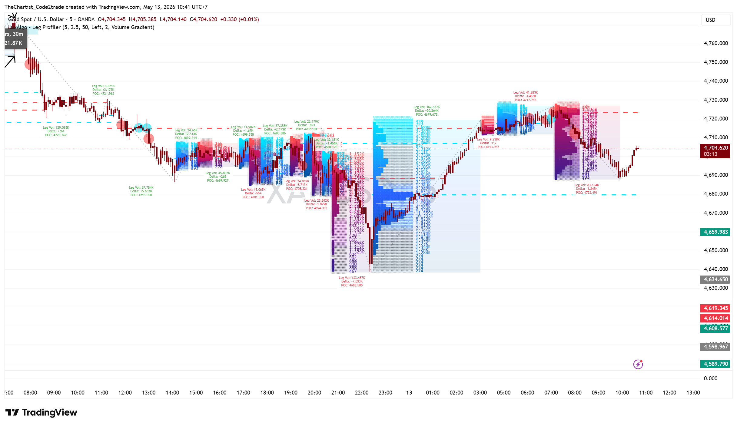
04 Structural Leg Profiler [LuxAlgo]
Isolated Scroll Container 1. Cup & Handle Indicator Description (Zeiierman) An indicator that automatically detects the Cup & Handle pattern – one of the most classic chart patterns in technical analysis 1.1 Indicator Concept The Cup & Handle indicator is based on the theory of market psychology patterns discovered by
03 Ranked FVG
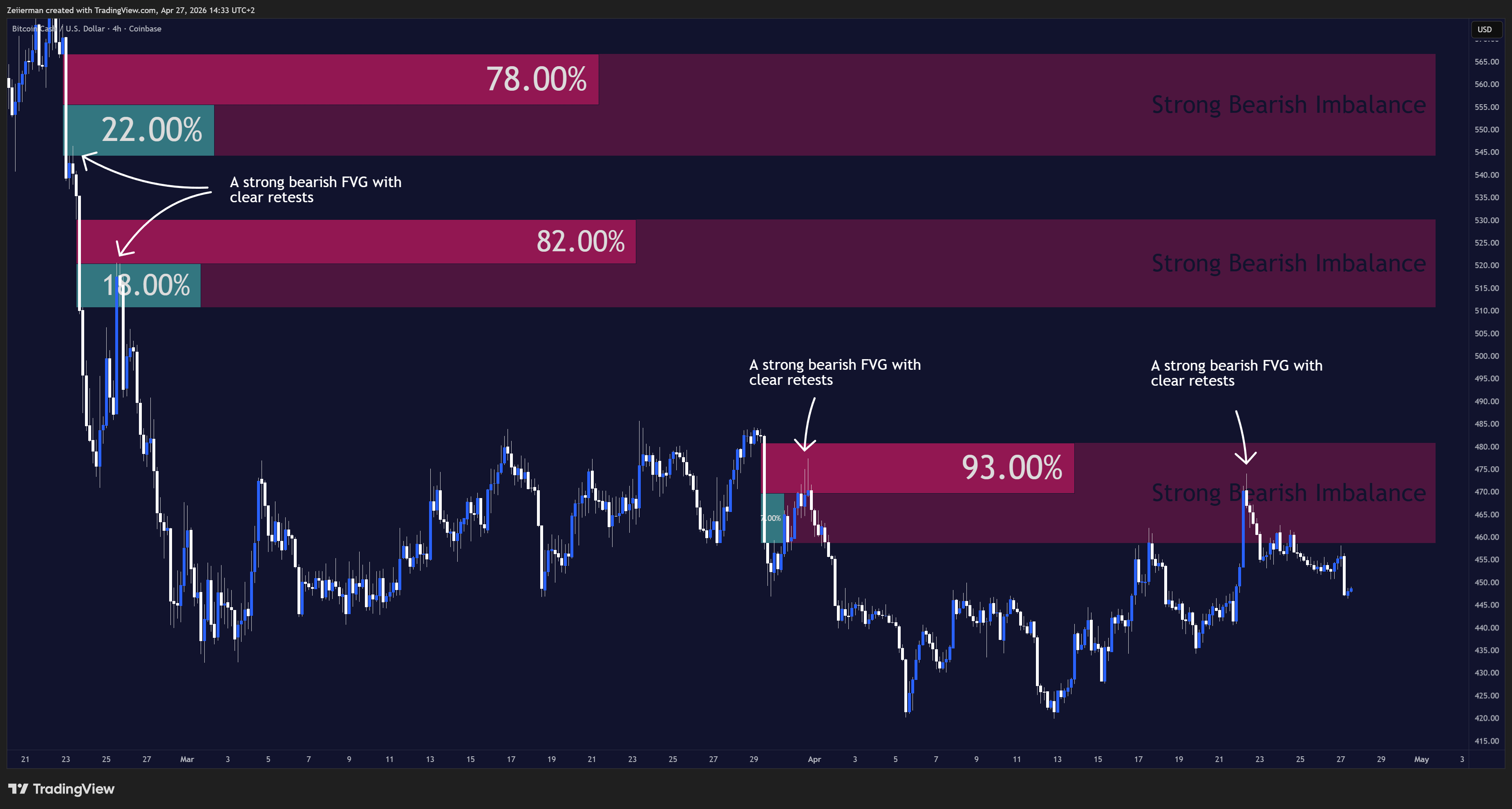
Isolated Scroll Container 1. Indicator Description – Ranked FVG Imbalance Zones (Zeiierman) Detects, ranks, and displays the highest-quality Fair Value Gap zones on the chart using a dynamic scoring system 1.1 Indicator Concept A Fair Value Gap (FVG) — also called a price imbalance — is a concept rooted in

Volume Divergence is fucking Trash!!
This isn’t just another lagging indicator. This strategy is a “Financial X-Ray” that combines Volume Delta with the precision of Trading Hub 3.0 to catch market reversals before they even hit the news