Machine Learning Moving Average TradingView indicator
A weighted moving average whose weights come out of Gaussian Process Regression, wrapped in an error band with a latching bull/bear state.
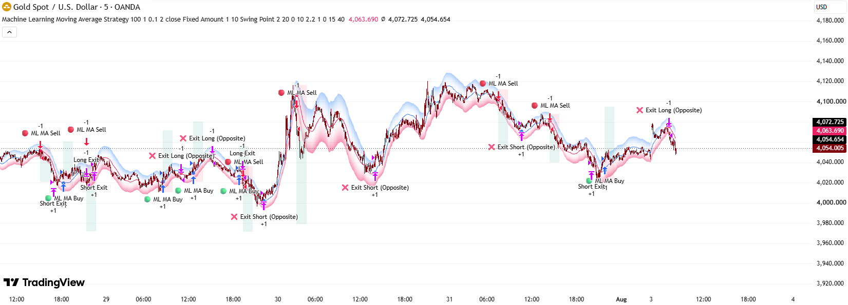
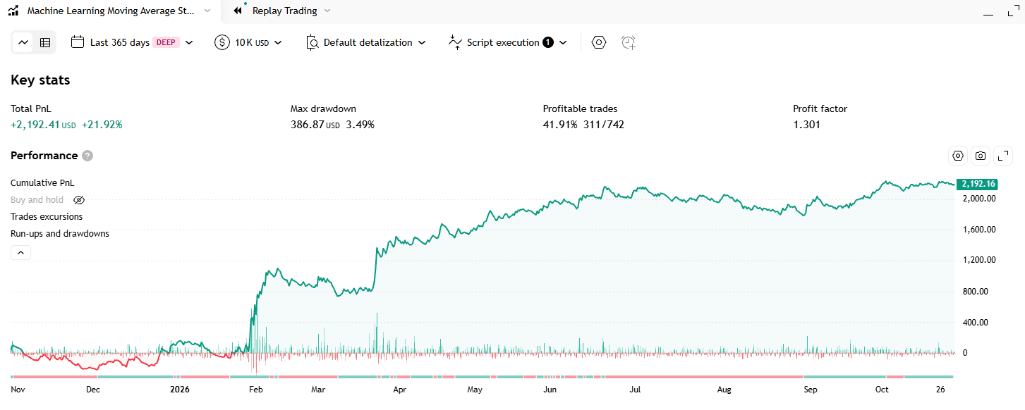
Quick summary: The Machine Learning Moving Average indicator draws a moving average whose per-bar weights are not picked by you but solved for with Gaussian Process Regression. Around that line sits a band two mean-absolute-errors wide, plus a bullish/bearish state that only flips when a close breaks outside the band in the same direction the line is already travelling. The strategy conversion was backtested over 365 days on gold (XAUUSD): 742 trades, 41.91% win rate, 1.301 profit factor, 3.49% maximum drawdown.
What is the Machine Learning Moving Average indicator? The idea behind it
Every moving average is a weighted sum. An SMA hands the last 100 bars identical weights; an EMA hands recent bars exponentially larger ones. Both of those weighting schemes were decided by a human and then frozen into a formula. This indicator asks a different question: what if the weights were solved for instead of assumed?
The answer comes from Gaussian Process Regression (GPR). Its founding assumption is that two points close together in time are tightly related, points further apart are loosely related, and that relatedness decays along a bell curve. Feed that assumption into the maths and you can solve for the weights that fit the data closely while staying smooth — rather than trading "fast but noisy" (a short MA) against "smooth but late" (a long MA), which is all a period setting ever lets you do.
A second assumption governs the band. The indicator measures how far price normally strays from the regression line and treats that distance as the baseline for ordinary noise. Movement inside it means nothing. Only when a close pushes clean outside the band and the regression line itself is already heading that way does the indicator call it a genuine change of regime. Requiring both halves at once is its entire filter against false signals.
If you are weighing up different ways to smooth price and read trend, the other regression channels and adaptive averages live in the Code2Trade free TradingView indicator library.
What Machine Learning Moving Average shows on the chart
Chart drawings
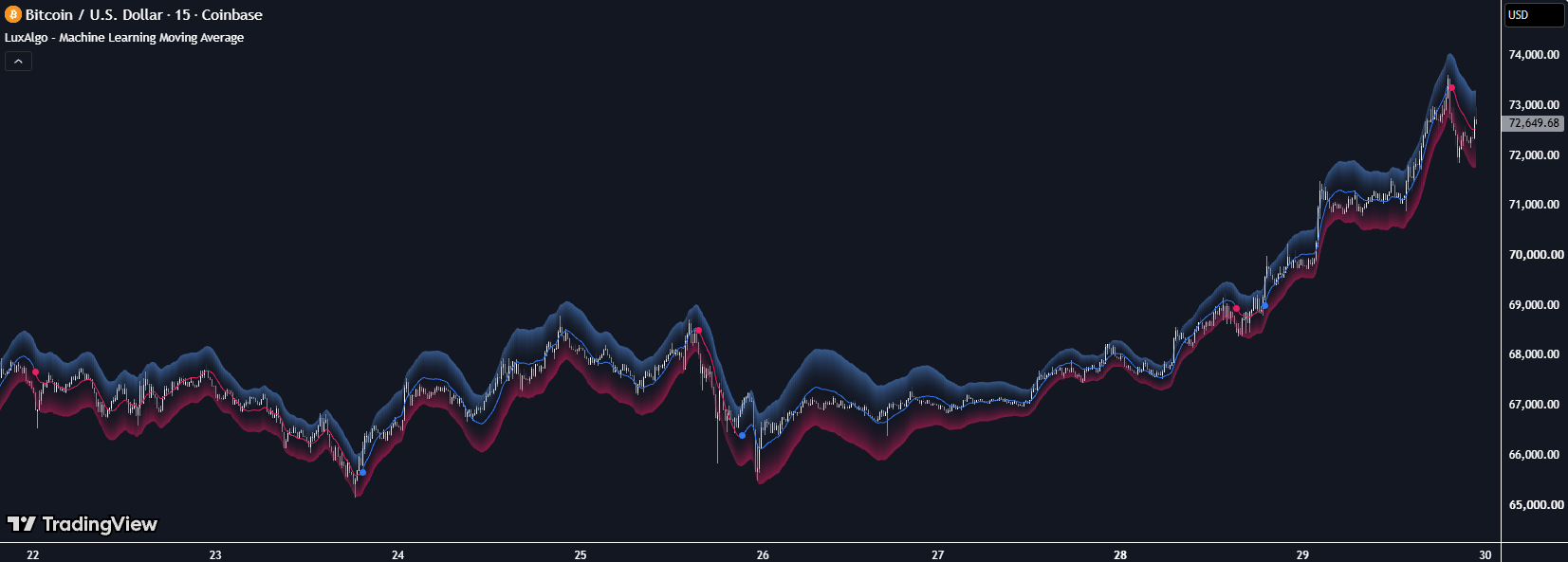
- The main "End Point GPR" line — the regression-built average, drawn over the price chart. It recolours with the state: blue while bullish, deep pink while bearish. The colour switches mid-line, with no wait for a leg to finish.
- A dot marking the flip — one fat circle on the exact bar where the state changed direction, in the colour of the new state. It is the only visual marker that says "right here, the picture changed".
- Two gradient fills — above the line a light blue wash that is strongest at the upper edge and fades back toward the line; below it a light pink one strongest at the lower edge. Neither edge is stroked as a visible line, so what you see is a halo hugging the average rather than two drawn boundaries.
Alerts
- The original indicator declares no alerts at all — there is no alertcondition() anywhere in the code. To be notified when the state flips you have to build an alert by hand in TradingView off the plotted series, or add the code yourself.
How to trade with the Machine Learning Moving Average line
Long setup
Wait for the blue dot — it prints when a close has cleared the upper edge while the regression line is also pointing up. Buying that bar usually means chasing a move that has already run, so the lower-risk version is to wait for price to pull back onto the regression line itself, which tends to act as a moving floor while the state is bullish. Put the stop below the band's lower edge: on gold around the 4,500 level the default band runs roughly 12 points either side, so the stop sits some 12–15 points away from the line. Take profit when the opposite pink dot appears, or at whatever multiple of risk you trade.
Short setup
The mirror image: a pink dot says a close has broken the lower edge while the line is heading down. Sell a bounce back into the line, stop above the band's upper edge, exit when the state flips blue again.
When NOT to use it
- Tight ranges. The state only flips on a close outside a band two average errors wide. Inside a consolidation price rarely manages that, so the line's colour can sit unchanged for hundreds of bars while the real trend turns over several times. The line still looks good; its colour has simply gone stale.
- The first ~200 bars of any chart. The line needs 100 bars before it produces anything, and the error band needs another 100 on top of that. Do not read signals at the left edge of a chart, or on a symbol where your broker only serves a few hundred bars of history.
- Do not walk the first input down to zero. Its stated minimum is 0, but entering exactly 0 throws an error and the indicator vanishes from the chart — details below.
This line tells you the underlying trend but says nothing about which price levels matter, so it pairs naturally with a structure or volume tool. You can also merge several TradingView indicators into one without coding (in Vietnamese).
How Machine Learning Moving Average works, from kernel to drawn line
The most surprising thing in the source: the "machine learning" part runs exactly once, on the first bar of the chart, and never again. The entire matrix-building block sits inside barstate.isfirst. What it produces is 100 numbers — and those same 100 numbers are reused on every remaining bar.
Inputs and what each one does
- window (integer, default 100): the most important setting, and it does four jobs at once — it sets how many bars are used for training, doubles as the width of the kernel function, serves as the lookback for the average, and serves as the lookback for the error. Drop it to 50 and the line tracks price more tightly with a narrower band and far more signals; push it to 200 and the line flattens out and signals become rare. ⚠️ Its stated minimum is 0, but entering 0 breaks the whole script: the code reads row number window + forecast − 1 of a matrix, which with both at 0 becomes row −1, an index that does not exist. (Layer 1 in the flowchart)
- forecast (integer, default 0): pushes the point the regression estimates out past the training window. At 0 it estimates the current point. Raise it to 5 and the indicator estimates a point five steps further right but still draws it on the current bar — so in practice the line leads price slightly, shedding lag at the cost of overshooting. (Layer 1)
- sigma (float, default 0.01): the noise added along the matrix diagonal before it is inverted. This is the valve that keeps the inversion stable: too small and the matrix sits close to singular, larger and the line follows price with a looser grip. Note the field steps in increments of 0.1 while its default is 0.01, so a single click of the up arrow jumps straight to 0.11 — eleven times the default. Fine adjustments have to be typed. (Layer 1)
- mult (float, default 2): multiplies the width of the error band. Halve it to 1 and the band narrows, flipping the state far more often; raise it to 3 and only violent breaks change the colour. This is the most intuitive sensitivity knob on the indicator. (Layer 1)
- src (price source, default close): the series the regression is fitted to. Switch it to hl2 for a slightly smoother line. (Layer 1)
- upCss / dnCss and bullCss / bearCss (colours): display only, they touch no calculation. The first pair fills the two bands, the second colours the line and the dot. (Layer 1)
The three fields window, forecast and sigma are declared without a title, so in the Settings dialog they appear as three unlabeled number boxes in exactly that order. The two line-colour swatches likewise share a single row carrying only the words "Moving Average".
Main calculation blocks
- Build the index scaffold. The indicator creates a list of positions 0, 1, 2 … 99 — these are bar numbers, not prices — plus a 100×100 identity matrix. (Layer 2 in the flowchart)
- Score how alike the positions are, with the rbf function. The formula is rbf(a,b) = exp(−(a−b)² / (2 × window²)): identical positions score exactly 1, and the score shrinks as they move apart. What stands out is that window is both the bar count and the denominator, which makes the scale very wide: the two furthest bars in the window, 99 apart, still score 0.61 alike. Every bar is strongly related to every other — which is precisely why the output line is so smooth. The result is two 100×100 matrices. (Layer 3)
- Invert the matrix — the one real training step. The indicator takes the pseudo-inverse of the kernel matrix. It is the heaviest computation in the script and the only part that deserves the word "training". (Layer 4)
- Extract 100 fixed weights. Multiply the two matrices and take a single row — the one matching the final point. Out comes a list of 100 numbers. The crucial part: that list depends only on window, forecast and sigma, and not at all on price. It is finished on the first bar and held unchanged to the end of the chart. (Layer 5)
- Apply the weights to price, once per bar. From here on everything repeats bar by bar. The indicator takes the 100-bar average, subtracts it from each price so only the deviation around zero is left, multiplies each deviation by its matching weight, sums them, then adds the average back. On gold: a 100-bar average of 4,498.0 plus a weighted sum of +9.4 puts the line at 4,507.4. The newest weight multiplies the current bar; the oldest multiplies the bar 99 candles back. (Layer 6)
- Measure the error and the direction. Take the absolute gap between price and the line, average it over 100 bars, multiply by mult — say an average error of 6.2 times 2 gives 12.4. Alongside that, the line is compared against its own previous value to see whether it is rising or falling. (Layer 7)
- Build the two edges. Upper edge = line + 12.4 = 4,519.8; lower edge = line − 12.4 = 4,495.0. (Layer 8)
- Latch the state. It turns bullish when a close clears 4,519.8 and the line is rising; bearish when a close breaks 4,495.0 and the line is falling. If neither fires, the previous state is kept — this is a remembered variable, not a comparison re-run from scratch each bar. A break of the band while the line has yet to turn therefore changes nothing. (Layer 9)
Outputs: drawings, orders, alerts
- The line and its colour are the main output: the line's position is the regression's idea of a fair value, the colour says which way the balance currently leans. (last layer in the flowchart)
- The dot is the only discrete signal — the marker you time an entry or exit off. (last layer)
- The two fills show the normal range of wandering, which is what makes them usable as stop placement. (last layer)
- There is no order output and no alert in the original indicator — automating it means converting it to a strategy first. (last layer)
What the one-time weight calculation means in practice: despite the name, this indicator learns nothing from the market while it runs. It is a fixed linear filter that differs from the familiar moving averages only in that its weights were solved out of GPR maths rather than chosen by a person. The upside is that it is cheap to run live — the expensive part was finished on bar one.
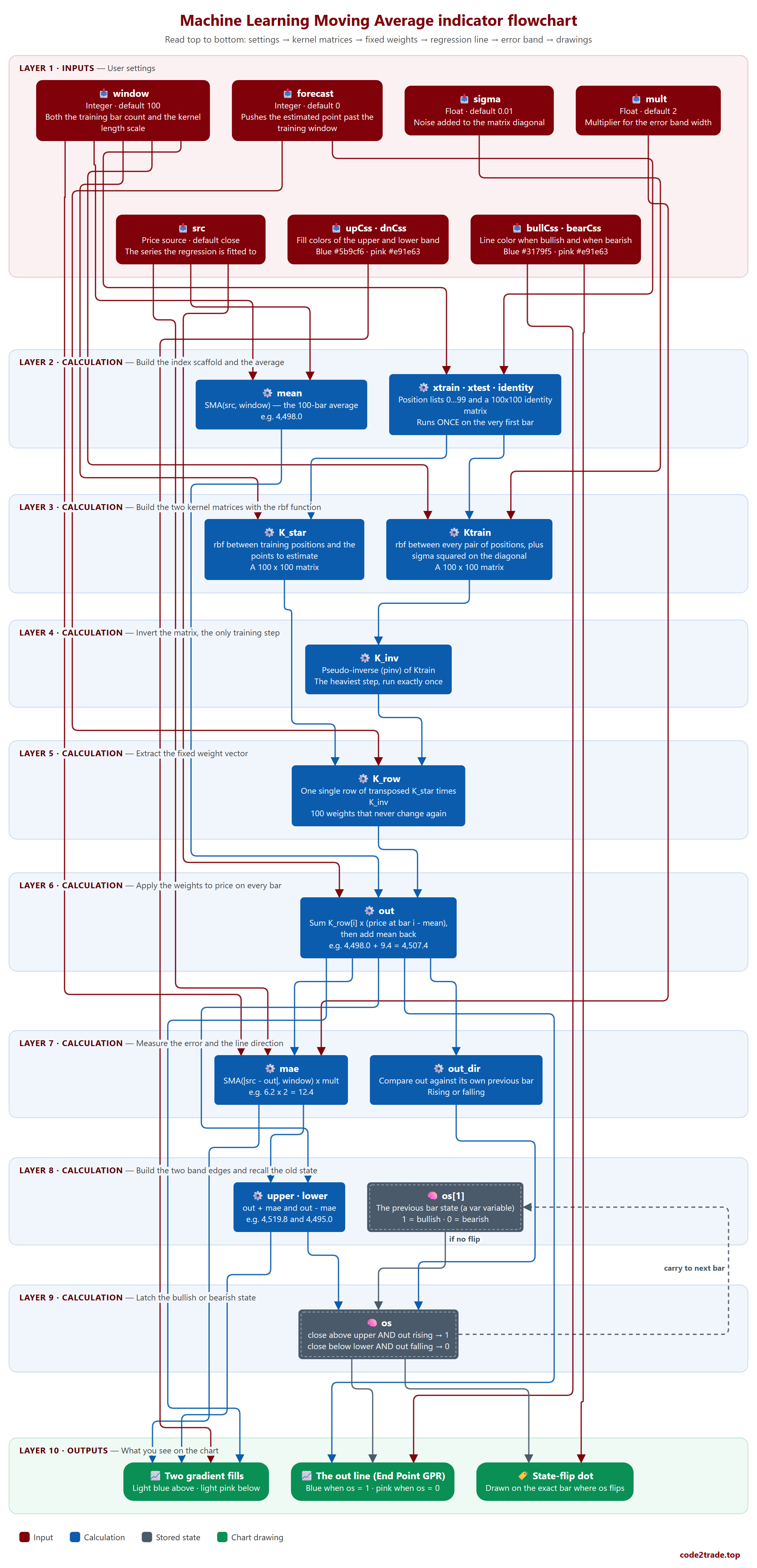
Machine Learning Moving Average flowchart, layer by layer

How to read the flowchart, layer by layer
Read the flowchart from top to bottom: the first four layers run exactly once on the very first bar to produce 100 weights; every later layer repeats on each bar using those same weights.
- Layer 1 — Inputs: User settings.
- window — an UNLABELED field in the Settings dialog. It feeds four places at once: the number of training positions, the l parameter of the rbf function, the mean lookback and the mae lookback. Setting it to 0 (its own minval) breaks the script outright. → leads to: xtrain · xtest · identity, mean, Ktrain, K_star, mae
- forecast — another unlabeled field. At the default 0 the regression estimates the current point; raising it estimates a point further to the right while still drawing it on the current bar. → leads to: xtrain · xtest · identity, K_row
- sigma — a third unlabeled field, with a step of 0.1 while the default is 0.01, so one click of the spinner jumps straight to 0.11. Larger values let the line follow price more loosely. → leads to: Ktrain
- mult — Float · default 2; Multiplier for the error band width → leads to: mae
- src — Price source · default close; The series the regression is fitted to → leads to: mean, out, mae
- upCss · dnCss — Fill colors of the upper and lower band; Blue #5b9cf6 · pink #e91e63 → leads to: Two gradient fills
- bullCss · bearCss — Line color when bullish and when bearish; Blue #3179f5 · pink #e91e63 → leads to: The out line (End Point GPR), State-flip dot
- Layer 2 — Calculation: Build the index scaffold and the average.
- xtrain · xtest · identity — these are bar position numbers, not prices. The whole block sits inside barstate.isfirst, so it runs exactly once for the entire chart. → leads to: Ktrain, K_star
- mean — this average is subtracted from price before the regression and added back at the end, so the regression only ever works with the deviation around zero. → leads to: out
- Layer 3 — Calculation: Build the two kernel matrices with the rbf function.
- Ktrain — rbf(a, b) = exp(-(a-b) squared / (2 x window squared)) measures how alike two positions are: the closer two bars sit, the nearer the value is to 1. Because window is both the bar count and the denominator, even the two furthest bars (99 apart) still score 0.61 alike, which is why the output line comes out so smooth. → leads to: K_inv
- K_star — rbf between training positions and the points to estimate; A 100 x 100 matrix → leads to: K_row
- Layer 4 — Calculation: Invert the matrix, the only training step.
- K_inv — the sigma added to the diagonal one layer above exists to keep this inversion stable; too small a sigma leaves the matrix close to singular. → leads to: K_row
- Layer 5 — Calculation: Extract the fixed weight vector.
- K_row — the row taken is number window + forecast - 1, the very last point. This weight vector depends only on window, forecast and sigma; it does not depend on price at all. → leads to: out
- Layer 6 — Calculation: Apply the weights to price on every bar.
- out — this is the main line you see on the chart. The newest weight multiplies the current bar and the oldest weight multiplies the bar 99 candles back. It only starts producing a value once the chart has run past window bars. → leads to: mae, out_dir, upper · lower, The out line (End Point GPR), Two gradient fills
- Layer 7 — Calculation: Measure the error and the line direction.
- mae — the average distance between price and the regression line over the last 100 bars, times mult. In a volatile market this number swells, the band widens and signals become rarer. → leads to: upper · lower, Two gradient fills
- out_dir — Compare out against its own previous bar; Rising or falling → leads to: os
- Layer 8 — Calculation: Build the two band edges and recall the old state.
- upper · lower — out + mae and out - mae; e.g. 4,519.8 and 4,495.0 → leads to: os, Two gradient fills
- os[1] — a var variable means the value is carried across bars instead of being recomputed. If this bar meets neither flip condition, the old state simply stays. → leads to: os (if no flip)
- Layer 9 — Calculation: Latch the bullish or bearish state.
- os — both halves are required to flip: breaking the band alone is not enough, the line direction has to agree. When neither fires the old state is kept, so os can sit unchanged for a long stretch. → leads to: The out line (End Point GPR), State-flip dot ↺ loops back to update (dashed): os[1] (carry to next bar)
- Layer 10 — Outputs: What you see on the chart.
- The out line (End Point GPR) — Blue when os = 1 · pink when os = 0
- State-flip dot — Drawn on the exact bar where os flips
- Two gradient fills — Light blue above · light pink below
This ten-layer diagram and the whole analysis above were produced with AI following the method taught in the Zero2Hero course: create indicators and trading bots using AI, no coding required.
Machine Learning Moving Average FAQ
Does it work for forex, gold or crypto?
So far it has only been tested on gold (XAUUSD), through the strategy conversion. Formula-wise the indicator uses no volume and is not tied to any session, so it will run on any symbol — but running and being profitable are separate claims. Forex pairs, crypto and stocks have not been backtested, so we make no claim about them.
Is the Machine Learning Moving Average indicator profitable?
The indicator on its own has no figures, because it draws rather than trades. The strategy conversion, backtested over 365 days on XAUUSD from 10,000 USD of capital, returned: 742 trades, 311 of them winners for a 41.91% win rate, +2,192 USD or +21.92%, a profit factor of 1.301, and a maximum drawdown of 386.87 USD or 3.49%. Read those numbers properly: a sub-50% win rate that still makes money means the average winner is bigger than the average loser, which is what a trend-following system should look like. A profit factor of 1.301 is modest — positive but not fat, and sensitive to the commission assumed.
Why call it machine learning if it is only a moving average?
Because the weights were solved with Gaussian Process Regression rather than chosen by hand. But to be straight about it: that solve runs exactly once on the first bar and yields 100 fixed numbers reused on every bar afterwards. The indicator learns nothing from new data while it runs. A more accurate description is a linear filter with machine-learning-derived weights, not an online learning model.
Is there an automated MT5 or OKX version?
The Pine Script strategy version exists; the MT5 build sits at a later stage of the workflow. In the meantime you can have AI connect to MetaTrader 5 in one click (in Vietnamese) and run the signal on your own account.
Can I get this indicator customised?
Yes — Code2Trade offers a custom TradingView indicator and trading bot coding service (Pine Script, MT5); send your request through the Code2Trade contact form.
For educational purposes only, not investment advice. Trading involves risk of loss.